Quick Start I: Local GUI

This notebook builds a Mach-Zehnder interferometer (MZI) from PDK cells in the local GUI and simulates it in Python, at no simulation cost.

In this notebook, you will learn how to:

• Open the local GUI from Python.

• Put the cells of an installed PDK in the Component Library.

• Draw a circuit in the schematic, then place and route it on the layout.

• Get the design from the GUI into Python.

• Simulate the circuit with free analytic models and plot its transmission.

You need PhotonForge and the open SiEPIC EBeam PDK:

pip install photonforge siepic-forge

This notebook runs no FDTD simulation and no mode solver, so it needs no Tidy3D account and uses no FlexCredits. To install PhotonForge, see Installation.

1. Import PhotonForge and set the PDK technology

Import PhotonForge and the SiEPIC EBeam PDK. Set the PDK technology as the default technology for new components.

import numpy as np
import photonforge as pf
import siepic_forge as siepic
from photonforge.live_viewer import LiveViewer

# Use the SiEPIC EBeam technology for new components
pf.config.default_technology = siepic.ebeam()

2. Open the local GUI

Start the local GUI. It runs on your computer, not in the cloud.

# Start the local GUI on port 8841
viewer = LiveViewer(port=8841)

LiveViewer started at http://127.0.0.1:8841. Call its 'stop()' method to free the port.

/home/lucas/Flexcompute/dev/photonforge-docs/.venv/lib/python3.10/site-packages/siepic_forge/component.py:53: RuntimeWarning: current config.grid does not exactly support the GDSII database unit; polygon vertices are snapped to config.grid
  c = pf.load_layout(fname, technology=technology)[cell_name]

Open http://localhost:8841 in your browser.

3. Build the MZI in the GUI

Do these steps in the browser. They take approximately two minutes.

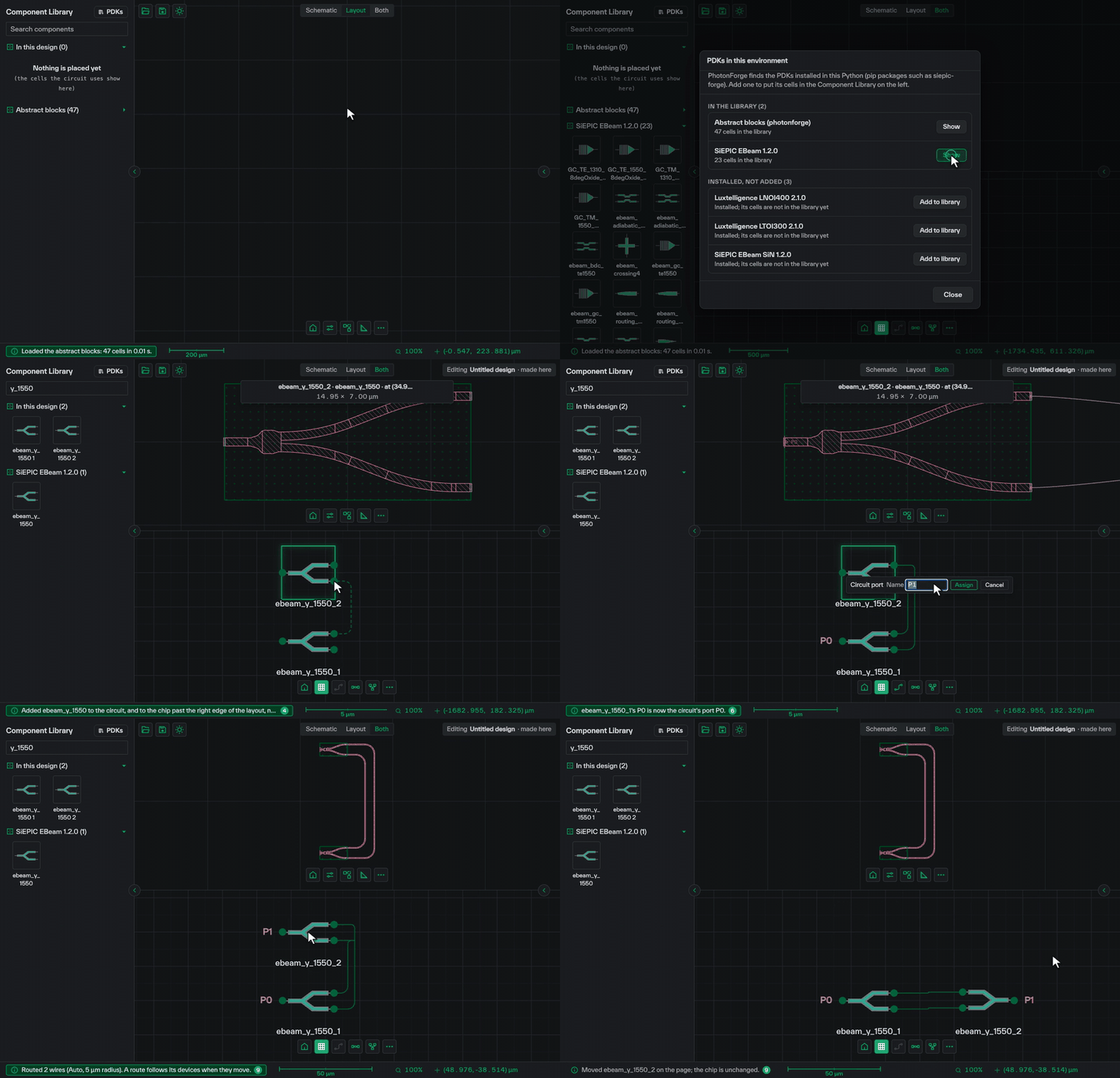
Put the SiEPIC EBeam cells in the Component Library:

1. Click PDKs at the top of the Component Library.

2. Click Add to library next to SiEPIC EBeam. If SiEPIC EBeam is under Not installed, click Install, or run pip install siepic-forge.

Draw the circuit in the schematic:

1. Click Both at the top of the page. The layout shows at the top and the schematic shows at the bottom.

2. Type y_1550 in Search components.

3. Drag the ebeam_y_1550 tile onto the schematic.

4. Drag the ebeam_y_1550 tile onto the schematic again, above the first Y-branch.

5. Drag a wire from the upper right port of the lower Y-branch to the lower right port of the upper Y-branch.

6. Drag a wire from the lower right port of the lower Y-branch to the upper right port of the upper Y-branch.

Make the input port and the output port of the circuit:

1. Right-click the left port of the lower Y-branch.

2. Click Assign port.

3. Click Assign. The name of this port is P0.

4. Do the same for the left port of the upper Y-branch. The name of this port is P1.

Make the layout:

1. Click Place, the third button on the toolbar under the layout.

2. Click Place in the box that opens.

3. Click Route, the third button on the toolbar under the schematic.

4. Type 5 in Bend radius.

5. Click Route.

On the layout, the two arms go to the right and fold back. The outer arm is longer than the inner arm, so the MZI is unbalanced.

Make the schematic read from left to right (this changes only the drawing, not the layout):

1. Click the upper Y-branch in the schematic.

2. Press R two times. The symbol turns 180 degrees. You can also right-click the symbol and click Rotate 90° two times.

3. Drag the symbol to the right of the lower Y-branch.

The schematic now shows P0, the splitter, the two arms, the combiner and P1, from left to right.

Turn a Y-branch only in the schematic, after Place. Place turns each device on the layout to match its symbol. If a device is turned on the layout, the circuit simulation solves the port modes to correct the phase, and the mode solver runs in the cloud.

4. Get the design into Python

The GUI changes the design in your Python session. viewer.component is the design that the GUI shows.

# Get the design that you built in the GUI
mzi = viewer.component
mzi

LayoutSchematic

Netlist

5. Use free models

The PDK cells come with Tidy3D FDTD models, and the routes come with models that use the mode solver. These models run in the cloud. For this first run, use analytic models. Analytic models run on your computer at no cost.

# Ideal 50/50 splitter model for the Y-branches
splitter_model = pf.PowerSplitterModel()

# Waveguide model with the typical n_eff and n_group of the 500 nm x 220 nm strip at 1550 nm
waveguide_model = pf.AnalyticWaveguideModel(n_eff=2.44, n_group=4.2)

Give the splitter model to each Y-branch and the waveguide model to each route. The waveguide model uses the length of the route.

# Give each instance in the design its analytic model
for reference in mzi.references:
    if reference.component.name == "ebeam_y_1550":
        reference.component.add_model(splitter_model, "Analytic")
    else:
        reference.component.add_model(waveguide_model, "Analytic")

6. Run the circuit simulation

A CircuitModel calculates the S matrix of the MZI from the models of its instances. pf.C_0 is the speed of light in µm/s, so pf.C_0 / wavelengths gives the frequencies.

# Calculate the S matrix of the MZI from 1500 nm to 1600 nm
mzi.add_model(pf.CircuitModel(), "Circuit")
wavelengths = np.linspace(1.5, 1.6, 1001)
s_matrix = mzi.s_matrix(pf.C_0 / wavelengths)

Progress: 100%

Plot the transmission from the input port P0 to the output port P1.

# Plot the transmission from P0 to P1 in dB
fig, ax = pf.plot_s_matrix(s_matrix, input_ports=["P0"], output_ports=["P1"], y="dB")

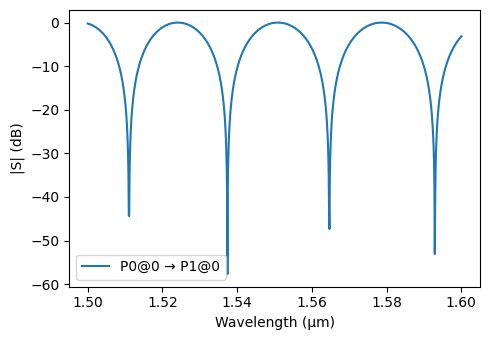
The transmission goes up and down with the wavelength because the two arms have different lengths. The distance between two dips is the free spectral range, FSR = λ² / (n_group ΔL). In this design, the arm length difference ΔL is approximately 21 µm, so the FSR is approximately 27 nm.

Optional: build the same MZI in Python

If you cannot use the GUI, build the MZI from a netlist. This cell uses the same cells and the same analytic models. The routes use the route function, not the auto router of the GUI. The outer arm uses a larger bend radius, so it goes around the inner arm. To simulate this MZI, use mzi_from_python in step 6.

# Build the MZI from a netlist, with the same cells and models
y_branch = siepic.component("ebeam_y_1550")
y_branch.add_model(splitter_model, "Analytic")

netlist = {
    "name": "MZI from Python",
    "instances": {"lower": y_branch, "upper": {"component": y_branch, "origin": (0, 56)}},
    "routes": [
        (("lower", "P2"), ("upper", "P1"), {"radius": 5, "model": waveguide_model}),
        (("lower", "P1"), ("upper", "P2"), {"radius": 10, "model": waveguide_model}),
    ],
    "ports": [("lower", "P0"), ("upper", "P0")],
    "models": [pf.CircuitModel()],
}
mzi_from_python = pf.component_from_netlist(netlist)
mzi_from_python

LayoutSchematic

Netlist

Next steps

Next, read the Circuit Model guide to simulate circuits with the PDK’s own Tidy3D models, which run in the cloud.