Directly Modulated Laser

The simplest optical transmitter has no modulator at all: the data drives the laser current directly. The price is that the laser’s own dynamics shape the signal, with turn-on delay, relaxation oscillations, a bias-dependent bandwidth, and frequency chirp. The DMLaserTimeStepper captures all of this by solving the single-mode semiconductor laser rate equations for the photon density \(p\), carrier density \(n\), and optical phase \(\phi\):

\[\frac{\mathrm{d} p}{\mathrm{d} t} = \Gamma G(p) (n - n_0) p - \frac{p}{\tau_p} + \frac{\beta \Gamma}{\tau_n} n \qquad \frac{\mathrm{d} n}{\mathrm{d} t} = \frac{I(t)}{q V_a} - G(p) (n - n_0) p - \frac{n}{\tau_n}\]

\[\frac{\mathrm{d} \phi}{\mathrm{d} t} = \frac{\alpha}{2} \left( \Gamma v_g a_0 (n - n_0) - \frac{1}{\tau_p} \right) \qquad G(p) = \frac{c_0}{n_g} \frac{a_0}{1 + \epsilon p}\]

with gain compression \(\epsilon\) and Henry’s linewidth enhancement factor \(\alpha\) coupling amplitude and phase. The electrical input amplitude is converted to the drive current as \(I = \Re \lbrace A \rbrace / \sqrt{Z_0}\), and the default parameters correspond to a textbook 1.55 µm semiconductor laser. The same intensity and phase noise mechanisms as the CW Laser are available through rel_intensity_noise and linewidth.

This guide measures the light-current characteristic, watches the turn-on dynamics, maps the modulation bandwidth against bias, and looks at the chirp that direct modulation imprints on the optical phase.

Reference

1. Coldren, L. A., Corzine, S. W., et al. Diode Lasers and Photonic Integrated Circuits. Wiley 2012.

2. Agrawal, G. P., Dutta, N. K. Semiconductor Lasers. Van Nostrand Reinhold 1993.

Setup

import matplotlib.pyplot as plt
import numpy as np
import photonforge as pf
import photonforge.abstract as pfa

viewer = pf.live_viewer.LiveViewer()

LiveViewer started at http://localhost:57866

tech = pf.basic_technology()
pf.config.default_technology = tech

f0 = pf.C_0 / 1.55  # optical carrier at 1.55 um
z0 = 50.0  # impedance of the electrical drive port
time_step = 0.5e-12  # fine enough to resolve the relaxation oscillations

The Light-Current Characteristic

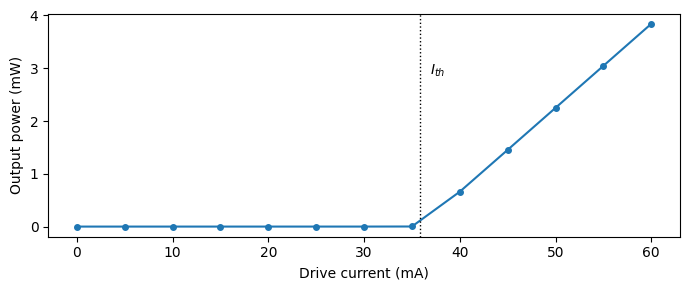
The abstract dm_laser has the electrical drive port E0 and the optical output P0. Sweeping a DC drive current from a signal_source (remembering that current maps to the wave amplitude as \(A = I \sqrt{Z_0}\)) and letting the rate equations settle at each point traces the LI curve: negligible spontaneous emission below threshold, then a linear rise with the slope efficiency set by quantum_efficiency. A linear fit of the above-threshold points gives the threshold current for reference.

# Laser with default (textbook 1.55 um diode) parameters
laser = pfa.dm_laser(seed=0)
viewer(laser)

# DC current source driving the laser; the optical output is the only circuit port
source = pfa.signal_source(amplitude=0, offset=0, seed=1)
link = pf.Component("dml_link")
laser_ref = link.add_reference(laser)
source_ref = link.add_reference(source)
source_ref.connect("E0", laser_ref["E0"])
link.add_port(laser_ref["P0"], "out")
link.add_model(pf.CircuitModel(), "Circuit")

# Sweep the DC current and record the settled output power at each point
currents = np.linspace(0, 60e-3, 13)
num_settle = 10000
power = []
for current in currents:
    # DC drive: current I maps to the amplitude I * sqrt(z0)
    source.update(offset=current * np.sqrt(z0))
    time_stepper = link.setup_time_stepper(
        time_step=time_step, carrier_frequency=f0, show_progress=False
    )
    a = time_stepper.step(steps=num_settle, time_step=time_step, show_progress=False)["out@0"]
    # Average the last nanosecond, well after the turn-on transient
    power.append(np.abs(a[-2000:]).mean() ** 2)
power = np.array(power)

# Threshold and slope efficiency from the above-threshold points
fit_mask = currents >= 45e-3
slope, intercept = np.polyfit(currents[fit_mask], power[fit_mask], 1)
i_threshold = -intercept / slope

fig, ax = plt.subplots(figsize=(7, 3), tight_layout=True)
ax.plot(currents * 1e3, power * 1e3, "o-", markersize=4)
ax.axvline(i_threshold * 1e3, color="k", linestyle=":", linewidth=1)
ax.text(i_threshold * 1e3 + 1, power.max() * 1e3 * 0.75, "$I_{th}$", fontsize=10)
ax.set(xlabel="Drive current (mA)", ylabel="Output power (mW)")

print(f"Threshold current: {i_threshold * 1e3:.1f} mA, slope efficiency: {slope:.3f} W/A")

Threshold current: 35.9 mA, slope efficiency: 0.159 W/A

Turn-On Dynamics

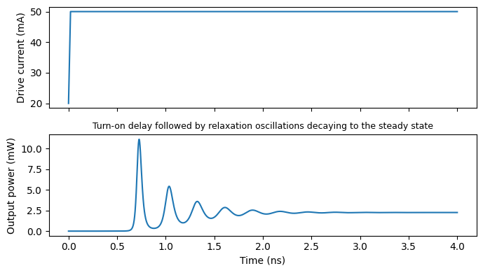
Stepping the current from below to above threshold shows the laser’s intrinsic dynamics at full scale. First comes the turn-on delay while the injected carriers fill the reservoir up to threshold, then the photon density overshoots and rings against the carrier population: the relaxation oscillations, which decay toward the steady state at the damping rate. Every large-signal property of a directly modulated link traces back to this response.

# Current step from 20 mA (below threshold) to 50 mA: a slow trapezoid
# with sharp edges holds each level long enough to see the full transient
i_low, i_high = 20e-3, 50e-3
source_step = pfa.signal_source(
    frequency=0.05e9,
    offset=i_low * np.sqrt(z0),
    amplitude=(i_high - i_low) * np.sqrt(z0),
    waveform="trapezoid",
    width=0.9,
    rise=0.001,
    fall=0.001,
    seed=1,
)
step_link = pf.Component("step_link")
laser_ref = step_link.add_reference(laser)
source_ref = step_link.add_reference(source_step)
source_ref.connect("E0", laser_ref["E0"])
step_link.add_port(laser_ref["P0"], "out")
step_link.add_model(pf.CircuitModel(), "Circuit")

# Monitor the laser's electrical port to plot the drive alongside the output
num_steps = 8000
t = np.arange(num_steps) * time_step
time_stepper = step_link.setup_time_stepper(
    time_step=time_step,
    carrier_frequency=f0,
    time_stepper_kwargs={"monitors": {"drive": laser_ref["E0"]}},
)
output = time_stepper.step(steps=num_steps, time_step=time_step)
power_step = np.abs(output["out@0"]) ** 2  # optical power from the envelope amplitude
current_step = np.real(output["drive@0-"]) / np.sqrt(z0)  # monitored current into the laser

fig, (ax1, ax2) = plt.subplots(2, 1, figsize=(7, 4), sharex=True, tight_layout=True)
ax1.plot(t * 1e9, current_step * 1e3)
ax1.set_ylabel("Drive current (mA)")
ax2.plot(t * 1e9, power_step * 1e3)
ax2.set(xlabel="Time (ns)", ylabel="Output power (mW)")
_ = ax2.set_title(
    "Turn-on delay followed by relaxation oscillations decaying to the steady state",
    fontsize=9,
)

Modulation Response vs Bias

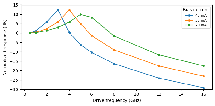
For small signals, the photon-carrier interplay behaves as a second-order resonance: the response is flat at low frequencies, peaks at the relaxation oscillation frequency \(f_R\), and falls steeply beyond it. Since \(f_R\) grows as \(\sqrt{I - I_{th}}\), biasing harder is the classic way to buy modulation bandwidth from a directly modulated laser.

We add a small sine on top of three bias currents and measure the tone in the output power at each drive frequency, normalizing every curve to its low-frequency value.

bias_currents = [45e-3, 55e-3, 70e-3]
drive_freqs = np.array([0.5e9, 1e9, 2e9, 3e9, 4e9, 5e9, 6e9, 8e9, 12e9, 16e9])
i_mod = 1e-3  # small modulation on top of the bias keeps the response linear

num_steps = 10000
t = np.arange(num_steps) * time_step
settled = slice(num_steps // 2, None)  # analyze only after transients die out

fig, ax = plt.subplots(figsize=(7, 3.5), tight_layout=True)
for bias in bias_currents:
    # Reuse the LI-curve circuit: only the source parameters change
    source.update(offset=bias * np.sqrt(z0), amplitude=i_mod * np.sqrt(z0))
    response = []
    for drive_freq in drive_freqs:
        source.update(frequency=drive_freq)
        time_stepper = link.setup_time_stepper(
            time_step=time_step, carrier_frequency=f0, show_progress=False
        )
        a = time_stepper.step(steps=num_steps, time_step=time_step, show_progress=False)["out@0"]
        p = np.abs(a) ** 2
        # Lock-in on the output power at the drive frequency
        tone = 2 * np.abs(
            np.mean((p[settled] - p[settled].mean()) * np.exp(-2j * np.pi * drive_freq * t[settled]))
        )
        response.append(tone)
    # Each curve is normalized to its own low-frequency response
    response = np.array(response)
    ax.plot(
        drive_freqs / 1e9,
        20 * np.log10(response / response[0]),
        "o-",
        markersize=4,
        label=f"{bias * 1e3:.0f} mA",
    )

source.update(amplitude=0)
ax.axhline(0, color="k", linewidth=0.5, alpha=0.5)
ax.set(xlabel="Drive frequency (GHz)", ylabel="Normalized response (dB)", ylim=(-30, 15))
_ = ax.legend(fontsize=8, title="Bias current")

Large-Signal Modulation and Chirp

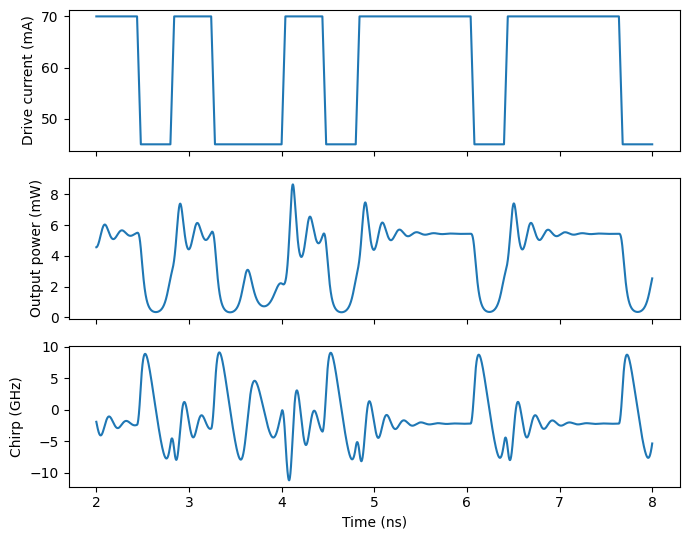
Driving the laser with data exposes the two large-signal signatures of direct modulation. The relaxation oscillations ring on every rising edge, and, through the \(\alpha\) factor, the carrier-density swings modulate the optical phase as well as the power: the output frequency spikes at the bit transitions (transient chirp) and settles to different values for ones and zeros (adiabatic chirp). The instantaneous frequency is read directly from the simulated envelope as \(\Delta f = (\mathrm{d} \phi / \mathrm{d} t) / 2 \pi\).

We drive a 2.5 Gb/s NRZ pattern between 45 and 70 mA. The chirp of several gigahertz that direct modulation imprints, much larger than the signal bandwidth, is what limits these transmitters over dispersive fiber, and why external modulators take over at higher rates and distances.

# 2.5 Gb/s NRZ pattern switching the current between 45 mA (zeros) and 70 mA (ones)
bit_rate = 2.5e9
source_data = pfa.signal_source(
    frequency=bit_rate,
    offset=45e-3 * np.sqrt(z0),
    amplitude=25e-3 * np.sqrt(z0),
    waveform="trapezoid",
    width=1.1,
    rise=0.1,
    fall=0.1,
    prbs=7,
    seed=1,
)
data_link = pf.Component("data_link")
laser_ref = data_link.add_reference(laser)
source_ref = data_link.add_reference(source_data)
source_ref.connect("E0", laser_ref["E0"])
data_link.add_port(laser_ref["P0"], "out")
data_link.add_model(pf.CircuitModel(), "Circuit")

num_steps = 20000
t = np.arange(num_steps) * time_step
time_stepper = data_link.setup_time_stepper(
    time_step=time_step,
    carrier_frequency=f0,
    time_stepper_kwargs={"monitors": {"drive": laser_ref["E0"]}},
)
output = time_stepper.step(steps=num_steps, time_step=time_step)
a = output["out@0"]
current_data = np.real(output["drive@0-"]) / np.sqrt(z0)

# Instantaneous frequency offset from the envelope phase
frequency_offset = np.gradient(np.unwrap(np.angle(a)), time_step) / (2 * np.pi)

# Show a few bits after the initial settling
window = (t > 2e-9) & (t < 8e-9)
fig, (ax1, ax2, ax3) = plt.subplots(3, 1, figsize=(7, 5.5), sharex=True, tight_layout=True)
ax1.plot(t[window] * 1e9, current_data[window] * 1e3)
ax1.set_ylabel("Drive current (mA)")
ax2.plot(t[window] * 1e9, np.abs(a[window]) ** 2 * 1e3)
ax2.set_ylabel("Output power (mW)")
ax3.plot(t[window] * 1e9, frequency_offset[window] / 1e9)
_ = ax3.set(xlabel="Time (ns)", ylabel="Chirp (GHz)")

Summary

• pfa.dm_laser solves the laser rate equations with the drive current taken from its electrical port as \(I = \Re \lbrace A \rbrace / \sqrt{Z_0}\); the default parameters describe a textbook 1.55 µm diode laser.

• The LI curve shows the threshold current and the slope efficiency set by quantum_efficiency.

• Large drive steps produce turn-on delay and relaxation oscillations; for small signals the same resonance sets the modulation bandwidth, with the peak frequency growing as \(\sqrt{I - I_{th}}\), so bias buys bandwidth.

• The linewidth_enhancement_factor couples the carrier dynamics into the optical phase, producing the transient and adiabatic chirp visible in the instantaneous frequency of the output.

• rel_intensity_noise and linewidth add the same noise mechanisms described in the CW Laser guide, and the physical parameters (photon_lifetime, carrier_lifetime, differential_gain, gain_compression_factor, and the rest) can all be matched to a specific device.