Analytic Dual-Ring Resonator Model

This guide covers pf.DualRingModel, which models two side-coupled ring resonators sharing an inter-ring coupling. The serially-coupled (second-order) topology produces a wider, flatter passband in the drop channel and steeper roll-off compared with a single ring, making it attractive for WDM add-drop filters and higher-order electro-optic modulators.

Device Topology

Two rings sit between two bus waveguides. The coupling coefficients are:

• kappa1: field coupling from Bus 1 into Ring 1.

• kappa2: field coupling between Ring 1 and Ring 2 (inter-ring).

• kappa3: field coupling from Ring 2 into Bus 2 (set kappa3=None for single-bus).

For the double-bus configuration the 4-port S-matrix is

\[\begin{split}S = \begin{bmatrix} 0 & t_1 & d & 0 \\\\ t_1 & 0 & 0 & d \\\\ d & 0 & 0 & t_2 \\\\ 0 & d & t_2 & 0 \end{bmatrix}\end{split}\]

where \(t_1\) and \(t_2\) are the through-port transmissions and \(d\) is the drop-port transmission. A signal entering at P0 (Bus 1 in) exits at P1 (Bus 1 out, through) and P2 (Bus 2 in, drop).

Transfer Functions

The round-trip field amplitude for ring \(i\) is

\[A_i(f) = 10^{-\alpha_i L_i/20}\,\exp\!\left(j\,\frac{2\pi}{c} \bigl[f\,n_{\mathrm{g},i}+f_0(n_{\mathrm{eff},i}-n_{\mathrm{g},i})\bigr]L_i\right)\]

where \(\alpha_i\) is the propagation loss in dB/µm, \(L_i\) the round-trip length, \(n_{\mathrm{eff},i}\) and \(n_{\mathrm{g},i}\) the effective and group indices, and \(f_0\) the reference frequency.

Each directional coupler with field coupling \(\kappa_i\) has a through-field

\[\tau_i = -j\,e^{j\angle\kappa_i}\sqrt{1-|\kappa_i|^2}\]

Through port

Ring 2 together with its bus coupler acts as an effective mirror seen by Ring 1. Collapsing Ring 2 + Bus 2 into \(\tau_{23}\):

\[\tau_{23} = \frac{\tau_2 - (\tau_2^2-\kappa_2^2)\,\tau_3\,A_2} {1 - \tau_2\,\tau_3\,A_2}\]

Then Ring 1 with that effective mirror gives the through-port transmission \(t_1\):

\[t_1 = \frac{\tau_1 - (\tau_1^2-\kappa_1^2)\,\tau_{23}\,A_1} {1-\tau_1\,\tau_{23}\,A_1}\]

Drop port

The drop-port transmission collects light that passes through all three couplers (\(\kappa_1\), \(\kappa_2\), \(\kappa_3\)) and half a round-trip in each ring:

\[d = \frac{\kappa_1\,\kappa_2\,\kappa_3\,A_1^{1/2}\,A_2^{1/2}} {1 - \tau_1\tau_2 A_1 - \tau_2\tau_3 A_2 + \tau_1\tau_3(\tau_2^2-\kappa_2^2)\,A_1 A_2}\]

These are the exact expressions used internally by pf.DualRingModel. For the single-bus case (kappa3=None) set \(\tau_3=1\), \(\kappa_3=0\).

import matplotlib.pyplot as plt
import numpy as np
import photonforge as pf
from photonforge.utils import C_0

pf.config.default_technology = pf.basic_technology()

C = C_0  # speed of light in µm/s

lam0 = 1.55  # µm
f0 = C / lam0
n_eff = 2.418
n_g = 4.2
L = 50.0  # µm
loss = 1e-3  # dB/µm

print(f"f0 = {f0:.4e} Hz")
print(f"FSR = {lam0**2/(n_g*L)*1e3:.2f} nm")

f0 = 1.9341e+14 Hz
FSR = 11.44 nm

Single Ring vs Dual Ring

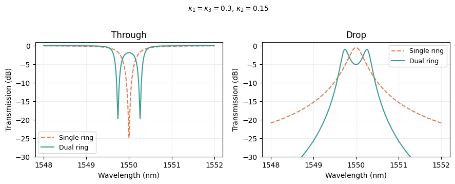
Compare a single add-drop ring with a dual-ring system having the same bus coupling strengths. The dual ring shows a wider drop passband and steeper edges.

lam = np.linspace(1.5480, 1.5520, 10001)
freqs = C / lam

# Single ring add-drop
single = pf.RingModel(
    kappa1=1j * 0.3,
    kappa2=1j * 0.3,
    n_eff=n_eff,
    n_group=n_g,
    length=L,
    propagation_loss=loss,
    reference_frequency=f0,
)
bb_single = single.black_box_component(port_spec="Strip")
s_single = bb_single.s_matrix(freqs)
thru_s = s_single[("P0@0", "P1@0")]
drop_s = s_single[("P0@0", "P2@0")]

# Dual ring (double-bus add-drop)
dual = pf.DualRingModel(
    kappa1=1j * 0.3,
    kappa2=1j * 0.15,
    kappa3=1j * 0.3,
    n_eff1=n_eff,
    n_eff2=n_eff,
    n_group1=n_g,
    n_group2=n_g,
    length1=L,
    length2=L,
    propagation_loss1=loss,
    propagation_loss2=loss,
    reference_frequency=f0,
)
bb_dual = dual.black_box_component(port_spec="Strip")
s_dual = bb_dual.s_matrix(freqs)
thru_d = s_dual[("P0@0", "P1@0")]
drop_d = s_dual[("P0@0", "P2@0")]

fig, axes = plt.subplots(1, 2, figsize=(9, 3.5))
for ax, T_single, T_dual, title in zip(
    axes,
    [thru_s, drop_s],
    [thru_d, drop_d],
    ["Through", "Drop"],
):
    ax.plot(
        lam * 1e3,
        10 * np.log10(np.abs(T_single) ** 2),
        color="#e07b54",
        ls="--",
        label="Single ring",
        lw=1.5,
    )
    ax.plot(
        lam * 1e3,
        10 * np.log10(np.abs(T_dual) ** 2),
        color="#3a9d92",
        label="Dual ring",
        lw=1.5,
    )
    ax.set_xlabel("Wavelength (nm)")
    ax.set_ylabel("Transmission (dB)")
    ax.set_title(title)
    ax.legend(fontsize=9)
    ax.set_ylim(-30, 1)
    ax.grid(True, alpha=0.2)

fig.suptitle(r"$\kappa_1=\kappa_3=0.3$, $\kappa_2=0.15$", y=1.01, fontsize=10)
fig.tight_layout()
plt.show()

Inter-ring Coupling kappa2 Sweep

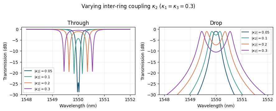
The inter-ring coupling strength kappa2 controls the eigenmode splitting. Larger kappa2 spreads the two resonance peaks further apart, widening the passband. Choosing kappa2 independently from the bus couplings lets the designer trade bandwidth for passband flatness.

kappa2_values = [0.05, 0.10, 0.20, 0.30]
colors = ["#1a5276", "#3a9d92", "#e07b54", "#8e44ad"]

fig, axes = plt.subplots(1, 2, figsize=(9, 3.5))

for k2_abs, color in zip(kappa2_values, colors):
    dual_v = pf.DualRingModel(
        kappa1=1j * 0.3,
        kappa2=1j * k2_abs,
        kappa3=1j * 0.3,
        n_eff1=n_eff,
        n_eff2=n_eff,
        n_group1=n_g,
        n_group2=n_g,
        length1=L,
        length2=L,
        propagation_loss1=loss,
        propagation_loss2=loss,
        reference_frequency=f0,
    )
    bb_v = dual_v.black_box_component(port_spec="Strip")
    s_v = bb_v.s_matrix(freqs)
    thru_v = s_v[("P0@0", "P1@0")]
    drop_v = s_v[("P0@0", "P2@0")]

    lbl = rf"$|\kappa_2|={k2_abs}$"
    axes[0].plot(
        lam * 1e3, 10 * np.log10(np.abs(thru_v) ** 2), color=color, label=lbl, lw=1.5
    )
    axes[1].plot(
        lam * 1e3, 10 * np.log10(np.abs(drop_v) ** 2), color=color, label=lbl, lw=1.5
    )

for ax, title in zip(axes, ["Through", "Drop"]):
    ax.set_xlabel("Wavelength (nm)")
    ax.set_ylabel("Transmission (dB)")
    ax.set_title(title)
    ax.legend(fontsize=8, loc="best")
    ax.set_ylim(-30, 1)
    ax.grid(True, alpha=0.2)

fig.suptitle(
    r"Varying inter-ring coupling $\kappa_2$ ($\kappa_1=\kappa_3=0.3$)", y=1.01
)
fig.tight_layout()
plt.show()

Flat-top Filter Response

A single add-drop ring has a Lorentzian (first-order) drop response. Two coupled rings produce two eigenmodes whose resonance frequencies straddle the individual ring resonance. With matched rings (\(L_1=L_2\), \(n_{\mathrm{eff},1}=n_{\mathrm{eff},2}\)) the result is a wider, flatter passband and steeper roll-off (second-order filter).

Maximally-Flat Design

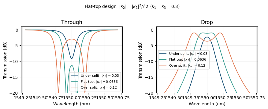
For a symmetric double-bus dual ring (\(\kappa_1 = \kappa_3\)), the maximally-flat (Butterworth) passband condition explained in this example is:

\[K_\mathrm{int} = \frac{1}{2}\,K_\mathrm{ext}^2\]

where \(K_\mathrm{ext} = |\kappa_1|^2 = |\kappa_3|^2\) and \(K_\mathrm{int} = |\kappa_2|^2\) are power coupling coefficients. In terms of the field coupling amplitudes passed to DualRingModel:

\[|\kappa_2| = \frac{|\kappa_1|^2}{\sqrt{2}}\]

This balances the eigenmode splitting against the linewidth so that the two resonance peaks merge into a single flat passband. Choosing \(|\kappa_2|\) smaller gives a single-peak (under-split) response; larger gives a double-peak (over-split) response.

# Flat-top design: |kappa2| = |kappa1|**2 / sqrt(2)
k_bus = 0.3  # |kappa1| = |kappa3| (field)
k2_flat = k_bus**2 / np.sqrt(2)  # flat-top condition (field)

k2_cases = [
    (0.03, r"Under-split, $|\kappa_2|=0.03$"),
    (k2_flat, rf"Flat-top, $|\kappa_2|={k2_flat:.4f}$"),
    (0.12, r"Over-split, $|\kappa_2|=0.12$"),
]
colors_ft = ["#1a5276", "#3a9d92", "#e07b54"]

lam_ft = np.linspace(1.5493, 1.5507, 50001)
freqs_ft = C / lam_ft

fig, axes = plt.subplots(1, 2, figsize=(9, 3.5))

for (k2, lbl), color in zip(k2_cases, colors_ft):
    m = pf.DualRingModel(
        kappa1=1j * k_bus,
        kappa2=1j * k2,
        kappa3=1j * k_bus,
        n_eff1=n_eff,
        n_eff2=n_eff,
        n_group1=n_g,
        n_group2=n_g,
        length1=L,
        length2=L,
        propagation_loss1=loss,
        propagation_loss2=loss,
        reference_frequency=f0,
    )
    bb = m.black_box_component(port_spec="Strip")
    s = bb.s_matrix(freqs_ft)
    thru_ft = s[("P0@0", "P1@0")]
    drop_ft = s[("P0@0", "P2@0")]
    axes[0].plot(
        lam_ft * 1e3,
        10 * np.log10(np.abs(thru_ft) ** 2),
        color=color,
        label=lbl,
        lw=1.5,
    )
    axes[1].plot(
        lam_ft * 1e3,
        10 * np.log10(np.abs(drop_ft) ** 2),
        color=color,
        label=lbl,
        lw=1.5,
    )

for ax, title in zip(axes, ["Through", "Drop"]):
    ax.set_xlabel("Wavelength (nm)")
    ax.set_ylabel("Transmission (dB)")
    ax.set_title(title)
    ax.legend(fontsize=8)
    ax.set_ylim(-20, 1)
    ax.grid(True, alpha=0.2)

fig.suptitle(
    r"Flat-top design: $|\kappa_2| = |\kappa_1|^2/\sqrt{2}$ "
    r"($\kappa_1=\kappa_3=0.3$)",
    y=1.01,
    fontsize=10,
)
fig.tight_layout()
plt.show()

Ring Detuning

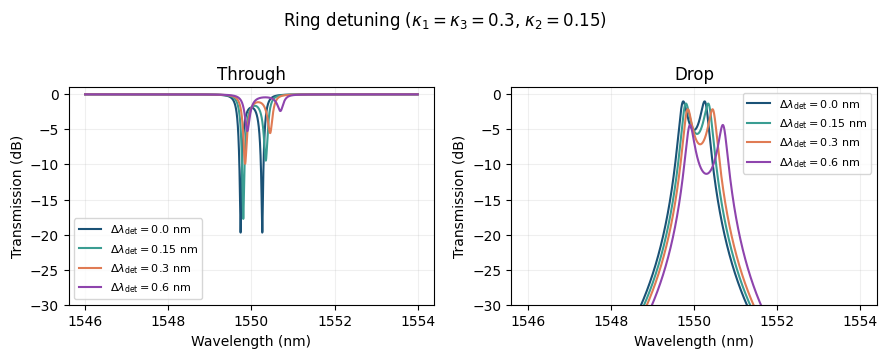
When the two rings have different effective indices, their resonances are offset. Detuning breaks the eigenmode symmetry: one peak couples more strongly to the drop port, and the passband splits into unequal peaks. At large detuning the rings effectively decouple. This can arise from fabrication variations or be introduced intentionally for dispersion engineering.

lam_det = np.linspace(1.5460, 1.5540, 10001)
freqs_det = C / lam_det

delta_nm_list = [0.0, 0.15, 0.30, 0.60]
colors_det = ["#1a5276", "#3a9d92", "#e07b54", "#8e44ad"]

fig, axes = plt.subplots(1, 2, figsize=(9, 3.5))

for delta_nm, color in zip(delta_nm_list, colors_det):
    dn_eff2 = n_g * (delta_nm * 1e-3) / lam0
    dual_det = pf.DualRingModel(
        kappa1=1j * 0.3,
        kappa2=1j * 0.15,
        kappa3=1j * 0.3,
        n_eff1=n_eff,
        n_eff2=n_eff + dn_eff2,
        n_group1=n_g,
        n_group2=n_g,
        length1=L,
        length2=L,
        propagation_loss1=loss,
        propagation_loss2=loss,
        reference_frequency=f0,
    )
    bb_det = dual_det.black_box_component(port_spec="Strip")
    s_det = bb_det.s_matrix(freqs_det)
    thru_det = s_det[("P0@0", "P1@0")]
    drop_det = s_det[("P0@0", "P2@0")]

    lbl = rf"$\Delta\lambda_{{\rm det}}={delta_nm}$ nm"
    axes[0].plot(
        lam_det * 1e3,
        10 * np.log10(np.abs(thru_det) ** 2),
        color=color,
        label=lbl,
        lw=1.5,
    )
    axes[1].plot(
        lam_det * 1e3,
        10 * np.log10(np.abs(drop_det) ** 2),
        color=color,
        label=lbl,
        lw=1.5,
    )

for ax, title in zip(axes, ["Through", "Drop"]):
    ax.set_xlabel("Wavelength (nm)")
    ax.set_ylabel("Transmission (dB)")
    ax.set_title(title)
    ax.legend(fontsize=8, loc="best")
    ax.set_ylim(-30, 1)
    ax.grid(True, alpha=0.2)

fig.suptitle(r"Ring detuning ($\kappa_1=\kappa_3=0.3$, $\kappa_2=0.15$)", y=1.01)
fig.tight_layout()
plt.show()

Single-bus (All-pass) Mode

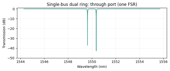
Setting kappa3=None removes the second bus waveguide. The result is a two-port all-pass filter whose through port shows two coupled resonance dips. This is useful as a notch filter or group-delay element.

FSR_nm = lam0**2 / (n_g * L) * 1e3
lam_fsr = np.linspace(lam0 - FSR_nm / 2 * 1e-3, lam0 + FSR_nm / 2 * 1e-3, 20001)
freqs_fsr = C / lam_fsr

# kappa1=0.15 gives near-critical coupling for deep resonance dips;
# kappa2=0.20 gives well-resolved splitting
dual_sb = pf.DualRingModel(
    kappa1=1j * 0.15,
    kappa2=1j * 0.20,
    kappa3=None,
    n_eff1=n_eff,
    n_eff2=n_eff,
    n_group1=n_g,
    n_group2=n_g,
    length1=L,
    length2=L,
    propagation_loss1=loss,
    propagation_loss2=loss,
    reference_frequency=f0,
)
bb_sb = dual_sb.black_box_component(port_spec="Strip")
s_sb = bb_sb.s_matrix(freqs_fsr)
thru_sb = s_sb[("P0@0", "P1@0")]

fig, ax = plt.subplots(figsize=(7, 3))
ax.plot(lam_fsr * 1e3, 10 * np.log10(np.abs(thru_sb) ** 2), color="#3a9d92", lw=1.5)
ax.set_xlabel("Wavelength (nm)")
ax.set_ylabel("Transmission (dB)")
ax.set_title(r"Single-bus dual ring: through port (one FSR)")
ax.set_ylim(-50, 1)
ax.grid(True, alpha=0.2)
fig.tight_layout()
plt.show()

Differential Thermal Tuning

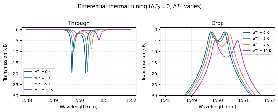
DualRingModel accepts independent temperatures temperature1 and temperature2 for each ring. For silicon, \(\mathrm{d}n/\mathrm{d}T \approx 1.85 \times 10^{-4}\) K\(^{-1}\), giving a resonance shift of roughly 0.068 nm/K. Tuning one ring relative to the other introduces a controlled detuning, allowing the passband shape to be reshaped dynamically after fabrication.

dn_dT = 1.85e-4  # Si thermo-optic coefficient, 1/K

lam_th = np.linspace(1.5480, 1.5520, 10001)
freqs_th = C / lam_th

dT1_values = [0, 2, 5, 10]
colors_th = ["#1a5276", "#3a9d92", "#e07b54", "#8e44ad"]

fig, axes = plt.subplots(1, 2, figsize=(9, 3.5))

for dT1, color in zip(dT1_values, colors_th):
    dual_th = pf.DualRingModel(
        kappa1=1j * 0.3,
        kappa2=1j * 0.15,
        kappa3=1j * 0.3,
        n_eff1=n_eff,
        n_eff2=n_eff,
        n_group1=n_g,
        n_group2=n_g,
        length1=L,
        length2=L,
        propagation_loss1=loss,
        propagation_loss2=loss,
        dn1_dT=dn_dT,
        dn2_dT=dn_dT,
        reference_frequency=f0,
        temperature1=293.0 + dT1,
        temperature2=293.0,
    )
    bb_th = dual_th.black_box_component(port_spec="Strip")
    s_th = bb_th.s_matrix(freqs_th)
    thru_th = s_th[("P0@0", "P1@0")]
    drop_th = s_th[("P0@0", "P2@0")]

    lbl = rf"$\Delta T_1={dT1}$ K"
    axes[0].plot(
        lam_th * 1e3,
        10 * np.log10(np.abs(thru_th) ** 2),
        color=color,
        label=lbl,
        lw=1.5,
    )
    axes[1].plot(
        lam_th * 1e3,
        10 * np.log10(np.abs(drop_th) ** 2),
        color=color,
        label=lbl,
        lw=1.5,
    )

for ax, title in zip(axes, ["Through", "Drop"]):
    ax.set_xlabel("Wavelength (nm)")
    ax.set_ylabel("Transmission (dB)")
    ax.set_title(title)
    ax.legend(fontsize=8, loc="best")
    ax.set_ylim(-30, 1)
    ax.grid(True, alpha=0.2)

fig.suptitle(
    r"Differential thermal tuning ($\Delta T_2=0$, $\Delta T_1$ varies)", y=1.01
)
fig.tight_layout()
plt.show()

Electro-optic Control

Like RingModel, DualRingModel supports voltage-dependent index modulation via dn1_dv, dn1_dv2, dn2_dv, dn2_dv2 for each ring independently. Each ring can also have voltage-dependent loss (dloss_dv_1, dloss_dv2_1, etc.).

For detailed EO modulation theory and examples, see the Analytic Ring Model guide.

Dual-ring electro-optic modulators are less common than single-ring designs, so we do not provide detailed examples here. The physics is straightforward: each ring independently shifts its resonance based on voltage, allowing differential phase or amplitude modulation across the two rings.

DualRingModel API Reference

Parameter	Type	Default	Notes
kappa1	complex	required	Bus 1 coupling (magnitude + phase)
kappa2	complex	required	Inter-ring coupling
kappa3	complex | None	None	Bus 2 coupling (None = single-bus)
n_eff1, n_eff2	float	required	Ring effective indices
n_group1, n_group2	float | None	n_eff	Group indices (defaults to n_eff)
length1, length2	float	required	Round-trip lengths (µm)
propagation_loss1, propagation_loss2	float	0.0	Loss (dB/µm)
reference_frequency	float | None	None	Taylor expansion point (Hz)
dn1_dT, dn2_dT	float	0.0	Thermo-optic coefficient (1/K)
temperature1, temperature2	float	293.0	Operating temperature (K)
dn1_dv, dn2_dv	float	0.0	Linear EO (1/V)
dn1_dv2, dn2_dv2	float	0.0	Quadratic EO (1/V\(^2\))
voltage1, voltage2	float	0.0	Operating voltage (V)

For more parameters (chromatic dispersion, loss temperature/voltage sensitivity, etc.), see the full pf.DualRingModel docstring.