Differentiator

Slopes carry information: the edges of a digital pattern mark its transitions, the derivative of a phase is a frequency, and the rate of change of a control signal feeds the D term of a PID loop. The abstract differentiator computes the scaled time derivative of an electrical signal, based on the DifferentialTimeStepper. Two finite-difference schemes are available:

\[y_k = s \, \frac{x_k - x_{k-1}}{\Delta t} \quad \text{(backwards)}, \qquad y_k = s \, \frac{x_k - x_{k-2}}{2 \Delta t} \quad \text{(central)}.\]

The scaling factor \(s\) is given in seconds, so the output is \(s \, dV/dt\): choosing \(s\) close to the time scale of the signal keeps the output amplitude comparable to the input. Together with the integrator and the expression-based blocks of the ExpressionTimeStepper, it completes the electrical math toolbox of the time-domain framework.

Setup

import matplotlib.pyplot as plt
import numpy as np
import photonforge as pf
import photonforge.abstract as pfa

viewer = pf.live_viewer.LiveViewer()

LiveViewer started at http://localhost:57571

tech = pf.basic_technology()
pf.config.default_technology = tech

f0 = pf.C_0 / 1.55
time_step = 1e-12
z0 = 50.0  # impedance of the virtual electrical ports

Differentiating a Pulse

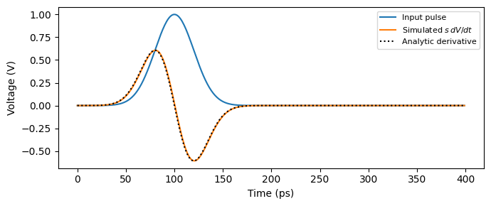
A Gaussian pulse makes the cleanest first test, since its derivative is known in closed form. The pulse is injected directly at the input port E0 and the derivative appears at E1. With the scale set to the pulse width \(s = \sigma\), the analytic result is

\[y(t) = -\frac{t - t_0}{\sigma} \, V_\mathrm{pk} \, e^{-(t - t_0)^2 / 2 \sigma^2},\]

a doublet with extrema of \(\pm V_\mathrm{pk} \, e^{-1/2}\) at \(t_0 \pm \sigma\), plotted below for reference. The backwards difference evaluates the slope between the current and the previous sample, so its output is the derivative at \(t - \Delta t / 2\): at this time step the half-sample shift is invisible on the plot.

sigma = 20e-12  # pulse width (s)
v_pk = 1.0  # pulse peak (V)
t0 = 100e-12

num_steps = 400
t = np.arange(num_steps) * time_step
pulse = v_pk / np.sqrt(z0) * np.exp(-((t - t0) ** 2) / (2 * sigma**2))

# Scale s = sigma keeps the output amplitude comparable to the input
differentiator = pfa.differentiator(scale=sigma)
time_stepper = differentiator.setup_time_stepper(
    time_step=time_step, carrier_frequency=f0, show_progress=False
)
out = time_stepper.step(
    inputs=pf.TimeSeries({"E0@0": pulse}, time_step), show_progress=False
)
derivative = np.real(out["E1@0"]) * np.sqrt(z0)

analytic = -(t - t0) / sigma * v_pk * np.exp(-((t - t0) ** 2) / (2 * sigma**2))

fig, ax = plt.subplots(figsize=(7, 3), tight_layout=True)
ax.plot(t * 1e12, pulse * np.sqrt(z0), label="Input pulse")
ax.plot(t * 1e12, derivative, label="Simulated $s \\, dV/dt$")
ax.plot(t * 1e12, analytic, "k:", label="Analytic derivative")
ax.set(xlabel="Time (ps)", ylabel="Voltage (V)")
_ = ax.legend(fontsize=8)

Bandwidth and Scheme Choice

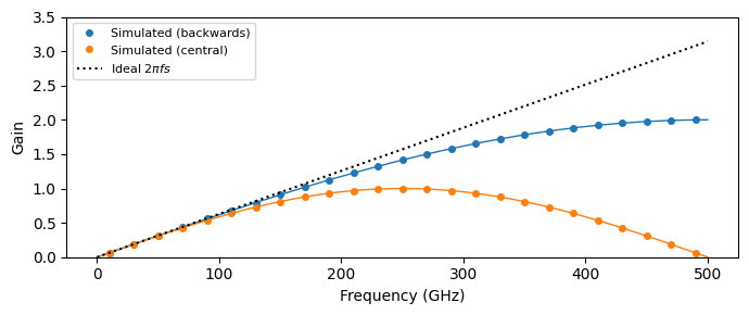
A finite difference only approximates the ideal response \(|H(f)| = 2 \pi f s\) at frequencies well below the Nyquist limit \(1 / (2 \Delta t)\). Evaluating the two schemes on a discrete tone gives

\[|H_\mathrm{bwd}(f)| = \frac{2 s}{\Delta t} \left| \sin(\pi f \Delta t) \right|, \qquad |H_\mathrm{ctr}(f)| = \frac{s}{\Delta t} \left| \sin(2 \pi f \Delta t) \right|,\]

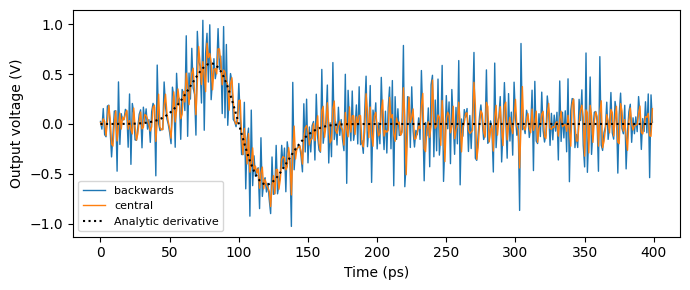
both plotted below against the measured gain from single-tone simulations. The backwards scheme follows the ideal ramp further and keeps growing up to Nyquist; the central scheme, being the average of two consecutive backwards differences, rolls off beyond a quarter of the sampling rate and returns to zero at Nyquist. That built-in high-frequency rejection is the reason to choose it: differentiation amplifies noise in proportion to frequency, and the central scheme caps that amplification.

num_steps = 4000
t = np.arange(num_steps) * time_step
frequencies = np.arange(10e9, 500e9, 20e9)  # integer GHz keeps FFT bins exact

fig, ax = plt.subplots(figsize=(7, 3), tight_layout=True)
scale = 1e-12
for scheme, color in [("backwards", "tab:blue"), ("central", "tab:orange")]:
    gains = []
    for frequency in frequencies:
        component = pfa.differentiator(scale=scale, scheme=scheme)
        time_stepper = component.setup_time_stepper(
            time_step=time_step, carrier_frequency=f0, show_progress=False
        )
        tone = np.sin(2 * np.pi * frequency * t)
        out = time_stepper.step(
            inputs=pf.TimeSeries({"E0@0": tone}, time_step), show_progress=False
        )
        # Tone amplitude at the output, read from its exact FFT bin
        bin_index = int(round(frequency * num_steps * time_step))
        gains.append(np.abs(np.fft.rfft(np.real(out["E1@0"]))[bin_index]) * 2 / num_steps)
    ax.plot(frequencies / 1e9, gains, "o", color=color, markersize=4, label=f"Simulated ({scheme})")

f_theory = np.linspace(0, 500e9, 500)
ax.plot(f_theory / 1e9, 2 * scale / time_step * np.abs(np.sin(np.pi * f_theory * time_step)),
        "-", color="tab:blue", linewidth=1)
ax.plot(f_theory / 1e9, scale / time_step * np.abs(np.sin(2 * np.pi * f_theory * time_step)),
        "-", color="tab:orange", linewidth=1)
ax.plot(f_theory / 1e9, 2 * np.pi * f_theory * scale, "k:", label="Ideal $2 \\pi f s$")
ax.set(xlabel="Frequency (GHz)", ylabel="Gain", ylim=(0, 3.5))
_ = ax.legend(fontsize=8)

The consequence is easy to see on a noisy signal: the same Gaussian pulse with a little white noise added comes out of the backwards differentiator buried in amplified noise, while the central scheme recovers a visibly cleaner derivative at no extra cost.

num_steps = 400
t = np.arange(num_steps) * time_step
rng = np.random.default_rng(seed=0)
noisy_pulse = pulse + 0.01 / np.sqrt(z0) * rng.standard_normal(num_steps)  # 10 mV RMS noise

fig, ax = plt.subplots(figsize=(7, 3), tight_layout=True)
for scheme in ["backwards", "central"]:
    component = pfa.differentiator(scale=sigma, scheme=scheme)
    time_stepper = component.setup_time_stepper(
        time_step=time_step, carrier_frequency=f0, show_progress=False
    )
    out = time_stepper.step(
        inputs=pf.TimeSeries({"E0@0": noisy_pulse}, time_step), show_progress=False
    )
    ax.plot(t * 1e12, np.real(out["E1@0"]) * np.sqrt(z0), label=scheme, linewidth=1)
ax.plot(t * 1e12, analytic, "k:", label="Analytic derivative")
ax.set(xlabel="Time (ps)", ylabel="Output voltage (V)")
_ = ax.legend(fontsize=8)

Application: Edge Detection

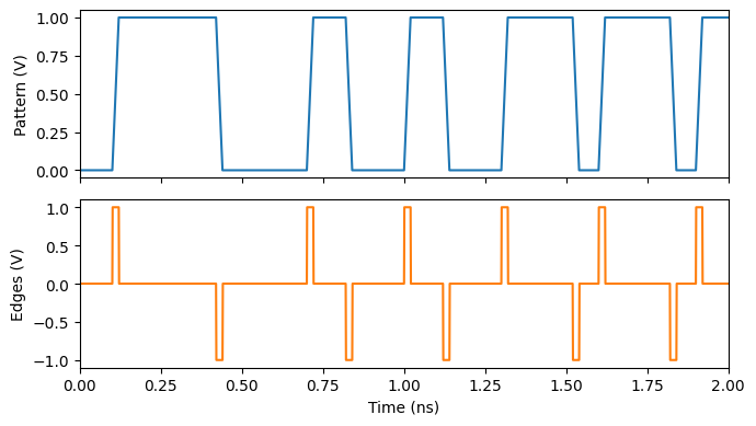
Differentiating a digital pattern turns its edges into pulses: rising transitions give positive spikes, falling ones negative, and flat stretches give nothing. This is the front end of clock-recovery and timing-analysis circuits. A 10 Gb/s NRZ pattern from the signal_source with 20 ps edges, differentiated with \(s = 20\) ps, produces spikes of the full swing amplitude at every transition.

num_steps = 3200
t = np.arange(num_steps) * time_step

# 10 Gb/s NRZ pattern with 20 ps rise and fall times
source = pfa.signal_source(
    waveform="trapezoid",
    amplitude=1.0 / np.sqrt(z0),
    frequency=10e9,
    prbs=7,
    width=1.2,
    rise=0.2,
    fall=0.2,
    seed=3,
)
source_stepper = source.setup_time_stepper(
    time_step=time_step, carrier_frequency=f0, show_progress=False
)
pattern = np.real(
    source_stepper.step(
        inputs=pf.TimeSeries({"E0@0": np.zeros(num_steps)}, time_step), show_progress=False
    )["E0@0"]
)

# Scale matched to the edge duration: a full-swing edge produces a full-swing spike
edge_detector = pfa.differentiator(scale=20e-12)
time_stepper = edge_detector.setup_time_stepper(
    time_step=time_step, carrier_frequency=f0, show_progress=False
)
out = time_stepper.step(
    inputs=pf.TimeSeries({"E0@0": pattern}, time_step), show_progress=False
)
edges = np.real(out["E1@0"]) * np.sqrt(z0)

fig, (ax1, ax2) = plt.subplots(2, 1, figsize=(7, 4), sharex=True, tight_layout=True)
ax1.plot(t * 1e9, pattern * np.sqrt(z0))
ax1.set(ylabel="Pattern (V)")
ax2.plot(t * 1e9, edges, color="tab:orange")
_ = ax2.set(xlabel="Time (ns)", ylabel="Edges (V)", xlim=(0, 2))

Summary

• pfa.differentiator outputs the scaled time derivative \(s \, dV/dt\) of the signal at its input port; the scale \(s\) is in seconds, and setting it near the signal time scale keeps amplitudes comparable.

• Two schemes are available: backwards (\((x_k - x_{k-1}) / \Delta t\)) follows the ideal \(2 \pi f s\) response closest to the Nyquist limit, while central (\((x_k - x_{k-2}) / 2 \Delta t\)) rolls off beyond a quarter of the sampling rate, capping the noise amplification inherent to differentiation.

• Both schemes are accurate for signals well below the Nyquist frequency, with sub-sample latency (half a sample for backwards, one sample for central).

• Differentiating a digital pattern is an edge detector: spikes mark the transitions, with sign indicating direction.

• The integrator provides the inverse operation, and the ExpressionTimeStepper covers memoryless custom math.