Quick Start III: Active

Quick Start II builds a passive Mach-Zehnder interferometer from a GDS layout and simulates it. Now we turn an MZI into a Mach-Zehnder modulator and run a complete 50 Gb/s transmitter link:

1. Load ready-made active components from a shared PhotonForge library.

2. Assemble the transmitter, letting the automatic router draw the waveguides.

3. Trim the interferometer with a thermal phase shifter and find its quadrature point.

4. Characterize the electro-optic modulator and measure its switching voltage.

5. Run a time-domain simulation of the full link and plot the eye diagram.

Everything here runs on your machine: the library’s components ship with their FDTD results already computed, and waveguide modes are solved locally.

Setup

import numpy as np
import photonforge as pf
import photonforge.abstract as pfa  # laser, sources, photodiode: models with no layout
import photonforge.pda as pda  # projects: load and share components
from matplotlib import pyplot as plt
from photonforge.live_viewer import LiveViewer

viewer = LiveViewer()  # interactive layout viewer, used to display each component

LiveViewer started at http://127.0.0.1:43385. Call its 'stop()' method to free the port.

Loading components from a shared library

Building a modulator from scratch means drawing doped rib waveguides, coplanar electrodes, and vias, and attaching a compact model to each. That is worth doing once; it is not worth doing on your first day.

PhotonForge projects can be shared, so the components can simply be handed to you. photonforge-quickstart-library is such a project, and it carries a Python module alongside its components. Importing that module gives you the parametric functions that generate them, so you can build each component at whatever parameters your design needs:

# Load the shared project. Nothing is copied into your account: you get a
# read-only view of its contents.
library = pda.load_project("photonforge-quickstart-library")

# A project can carry a Python module alongside its components. Importing it
# gives us the functions that generate those components, so we can build them at
# any parameters we like instead of being stuck with one fixed version.
modules = library.import_module(globals())

print("Library module:", library.module_name)

Library module: photonforgequickstartlibrary

Passing globals() imports the module into this notebook exactly as import photonforgequickstartlibrary would, so we can give it a short alias and look inside:

qs = photonforgequickstartlibrary

print("Module contents:", ", ".join(n for n in dir(qs) if not n.startswith("_")))

Module contents: cpw_modulator, gap_center, mzm_components, mzm_transmitter, pda_components, pda_technologies, thermal_phase_shifter, y_splitter

Three of those names are the parametric functions we care about:

function	what it builds
qs.cpw_modulator(length, v_pil, f_3db)	two doped rib phase shifters driven by a coplanar waveguide electrode
qs.thermal_phase_shifter(length, temperature)	a strip waveguide with a heater on top, carrying a thermo-optic model
qs.mzm_transmitter(...)	the whole transmitter, ready made

We will use the first two and assemble the transmitter ourselves, so that the routing step is visible rather than hidden inside a function.

The rest are supporting values: qs.gap_center is the offset of each optical arm from the electrode center line, and qs.y_splitter is the Y splitter from Quick Start II, stored in the project as a fixed component rather than a function. It arrives with its FDTD S parameters already computed and stored as a DataModel, which is why nothing in this notebook needs the cloud:

# The Part 1 Y splitter is available as a module component
viewer(qs.y_splitter)

The electro-optic modulator

For high-speed modulation the library provides a push-pull depletion-mode modulator: a reverse-biased PN junction across a rib waveguide in each arm, driven through a coplanar waveguide (CPW) electrode.

Both arms are active and identical, with the junction of the lower arm mirrored so that both p-sides face the central signal electrode. Each arm carries the electro-optic term v_piL (the modulation efficiency you would take from foundry documentation or extract from a charge simulation) plus a PhaseModTimeStepper for the time domain, including a first-order electrical bandwidth:

# The modulator is a parametric component (function).
# Default: 500 um long arms, VpiL = 2000 V.um, and a 40 GHz electrical bandwidth
modulator = qs.cpw_modulator()

viewer(modulator)  # CPW electrode down the middle, one doped rib arm on each side

LayoutSchematic

The thermal phase shifter

A resistive heater over a waveguide changes the silicon refractive index through the thermo-optic effect, which shifts the optical phase. It is far slower than an electro-optic modulator, which makes it the natural way to trim a bias point rather than to carry data.

# Default length is 50 um and the default temperature is 293 K (no heating yet)
heater = qs.thermal_phase_shifter()

viewer(heater)  # waveguide, the heater strip above it, and two probe pads

Its behavior comes from an AnalyticWaveguideModel. Printing the model shows every knob it exposes, including the thermo-optic coefficient dn_dT and the temperature we are going to sweep. Because these are model parameters rather than geometry, changing them costs nothing and touches no layout:

# The heater uses an analytic model that we can control at circuit level
print(repr(heater.active_model))

AnalyticWaveguideModel(length=50.0, n_eff=2.43987, propagation_loss=0.0, extra_loss=0.0, n_group=4.181079, dispersion=0.0, dispersion_slope=0.0, reference_frequency=193414489032258.06, dn_dT=0.000186, dL_dT=0.0, temperature=293.0, reference_temperature=293.0, voltage=0.0, v_piL=None, k2=0.0, k3=0.0, dloss_dv=0.0, dloss_dv2=0.0, absorption=None, confinement_factor=1.0, chirp=0.0)

Assembling the transmitter

Now we put the pieces together: the Y splitter as splitter and combiner, the heater in the lower arm, and the modulator across both arms. Each piece is placed relative to the one before it, using the bounding-box attributes (x_max, x_min) that every reference exposes, so the layout stays correct if a component’s length changes.

The interesting part is the wiring. Rather than drawing five waveguides by hand, we hand route_auto two matched lists of ports and let it find the paths, bending around whatever is in the way. collision_layers tells it which layer counts as an obstacle, so it avoids the silicon it must not cross while ignoring the metal and doping layers of the modulator:

def build_transmitter():
    mzm = pf.Component("mzm")

    # The Y splitter, used twice: once as splitter, once as combiner.
    # The combiner is the same component rotated to face the other way.
    splitter = mzm.add_reference(qs.y_splitter)
    combiner = mzm.add_reference(qs.y_splitter)

    # The heater sits in the lower arm only: that is what makes the bias adjustable.
    # gap_center is the offset of each optical arm from the CPW center line.
    h = mzm.add_reference(qs.thermal_phase_shifter())
    h.translate((splitter.x_max + 50, -qs.gap_center))

    # The modulator spans both arms, centered on the same axis as the splitters
    m = mzm.add_reference(qs.cpw_modulator())
    m.x_min = h.x_max + 50

    combiner.rotate(180)
    combiner.x_min = m.x_max + 50  # far end of the interferometer

    # Five connections to make, given as two matched lists: net1[i] joins net2[i].
    # Reading them in pairs: splitter upper output -> modulator upper input,
    # splitter lower output -> heater, heater -> modulator lower input, and the
    # two modulator outputs -> the combiner inputs.
    net1 = [(splitter, "P2"), (splitter, "P1"), (h, "P1"), (m, "P1"), (m, "P3")]
    net2 = [(m, "P0"), (h, "P0"), (m, "P2"), (combiner, "P1"), (combiner, "P2")]
    routes = pf.parametric.route_auto(
        port1=net1,
        port2=net2,
        radius=10,  # minimum bend radius the router may use (um)
        collision_layers=["Si"],  # treat only silicon as an obstacle
    )
    mzm.add_reference(routes)

    # Expose the outside world: optical in and out, plus the two push-pull drives
    mzm.add_port([splitter["P0"], combiner["P0"], m["E0"], m["E1"]])

    # A circuit model gathers the models of everything above and cascades them
    mzm.add_model(pf.CircuitModel())
    return mzm


mzm = build_transmitter()
viewer(mzm)

LayoutSchematic

Netlist

Trimming the interferometer with the heater

Sweeping the heater temperature shifts the phase of the lower arm and moves the interferometer along its transfer curve. Nothing needs rebuilding for the sweep: model_kwargs overrides model parameters at simulation time, and the override reaches the heater’s model wherever it sits in the hierarchy.

We look for the quadrature point, where transmission is half of its maximum and the response is steepest and most linear:

# Solve waveguide modes on this machine instead of in the cloud. Each routed
# waveguide needs a mode solution, and locally there's no FC cost.
pf.config.use_local_mode_solver = True

# Wavelength grid for the frequency-domain sweeps, and the matching frequencies.
# PhotonForge always takes frequencies, so we convert once here.
wavelengths = np.linspace(1.53, 1.57, 41)
freqs = pf.C_0 / wavelengths

# Index closest to 1.55 um in the wavelength array
lda_index = np.argmin(np.abs(wavelengths - 1.55))

# Sweep the heater from room temperature to 50 K above it
temperatures = np.linspace(293, 343, 51)
transmission_t = np.empty_like(temperatures, dtype=float)

for i, t in enumerate(temperatures):
    print(f"Computing: {t} K...", flush=True, end="\n" if t == temperatures[-1] else "\r")

    # model_kwargs overrides model parameters for this one call: no rebuilding.
    # It reaches the heater's model wherever it sits in the hierarchy.
    s = mzm.s_matrix(freqs, show_progress=False, model_kwargs={"temperature": t})
    # |S21|^2 is the optical power fraction reaching the output at 1.55 um
    power_transmission = np.abs(s[("P0@0", "P1@0")]) ** 2
    # Record the transmission at 1.55 um
    transmission_t[i] = power_transmission[lda_index]

# Quadrature is where transmission is half of maximum: the steepest, most linear
# point of the transfer curve, and the usual place to bias a modulator
half_max = 0.5 * transmission_t.max()
t_quad = temperatures[np.argmin(np.abs(transmission_t - half_max))]

plt.figure(figsize=(7, 4))
plt.plot(temperatures - 293, transmission_t)
plt.axvline(
    t_quad - 293, color="gray", ls="--", label=f"quadrature (dT = {t_quad-293:.0f} K)"
)
plt.axhline(half_max, color="gray", ls=":")
plt.xlabel("Heater temperature rise (K)")
plt.ylabel("Transmission at 1.55 um")
plt.legend()
plt.grid(True, alpha=0.3)
plt.show()

print(f"Quadrature at dT = {t_quad - 293:.1f} K")

Computing: 343.0 K...

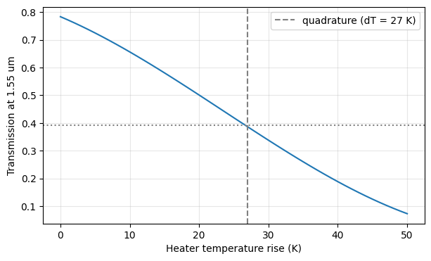
Quadrature at dT = 27.0 K

Two things are worth reading off that curve.

The peak transmission is below 1 because the splitter, the combiner, and the strip-to-rib tapers all lose a little light, and those losses come from the components’ own simulated S parameters rather than from any number we typed in.

More usefully, quadrature falls only about 3 K above room temperature. The two arms are nearly balanced by construction, so the unpowered device already sits close to the steep part of its transfer curve. That means we can leave the heater off for the rest of this notebook and let the electrical drive set the operating point; on a real chip the heater is what absorbs the fabrication spread that would otherwise move this curve.

Assembling the link

For the drive and the receiver we use PhotonForge’s abstract component library: a CW laser, two complementary NRZ sources, and a photodiode receiver. The push-pull drive works like a real dual-drive transmitter: one source carries the data pattern and the other carries its logical complement, so the phases of the two arms always move in opposite directions.

The link is assembled with component_from_netlist using virtual connections, which wire ports logically without requiring any physical layout:

f0 = pf.C_0 / 1.55  # optical carrier frequency: C_0 is in um/s, so 1.55 um -> Hz

z0 = 50.0  # impedance the electrical drives are referenced to (ohm)

bit_rate = 50e9  # 50 Gb/s NRZ
steps_per_bit = 160
time_step = 1 / (bit_rate * steps_per_bit)

# Each arm needs Vpi = VpiL / length to swing a full pi of phase. Because the two
# arms are driven oppositely, half of that on each arm switches the interferometer.
v_pi = 2000.0 / 500.0

# Time-domain electrical signals are waves in sqrt(W), so volts are divided by sqrt(z0)
drive = (v_pi / 2) / np.sqrt(z0)

# A random 128-bit pattern, and its logical complement for the second arm
num_bits = 128
rng = np.random.default_rng(seed=1)
bits = rng.integers(0, 2, num_bits)
bits_bar = 1 - bits

# Continuous-wave laser at the carrier frequency, 1 mW into the modulator
laser = pfa.cw_laser(power=1e-3, frequency=f0)

# The two drives. Trapezoidal bits with 10% rise and fall times are closer to a
# real driver than ideal square edges; width=1.1 slightly overlaps neighboring
# bits, as a bandwidth-limited driver does.
source_a = pfa.signal_source(
    frequency=bit_rate,
    amplitude=drive,
    offset=0,
    waveform="trapezoid",
    rise=0.1,
    fall=0.1,
    width=1.1,
    bit_sequence=bits,
)
source_b = pfa.signal_source(
    frequency=bit_rate,
    amplitude=drive,
    offset=0,
    waveform="trapezoid",
    rise=0.1,
    fall=0.1,
    width=1.1,
    bit_sequence=bits_bar,
)

# Receiver: 1 A/W photodiode into a 50 V/A transimpedance stage, 40 GHz bandwidth
photodiode = pfa.photodiode(responsivity=1.0, gain=50.0, filter_frequency=40e9)

link = pf.component_from_netlist(
    {
        "name": "mzm_link",
        "instances": {
            "laser": {"component": laser, "origin": (-50, 20)},
            "mzm": {"component": mzm, "origin": (0, 0)},
            "source_a": {"component": source_a, "origin": (500, 200)},
            "source_b": {"component": source_b, "origin": (500, -200)},
            "pd": {"component": photodiode, "origin": (1200, -20)},
        },
        # Virtual connections wire ports logically, with no waveguide or wire drawn.
        # The laser feeds the modulator, the two sources drive the two arms, and the
        # modulator output goes to the photodiode.
        "virtual connections": [
            (("laser", "P0"), ("mzm", "P0")),
            (("source_a", "E0"), ("mzm", "E0")),
            (("source_b", "E0"), ("mzm", "E1")),
            (("mzm", "P1"), ("pd", "P0")),
        ],
        # The only port we watch from outside is the receiver output
        "ports": [("pd", "E0", "RX_OUT")],
        "models": [(pf.CircuitModel(), "Circuit")],
    }
)

viewer(link)

LayoutSchematic

DC modulation transfer

First we characterize the modulator statically, exactly like on a bench: set both sources to complementary DC offsets, run a short time-domain simulation, and record the settled receiver output.

The result is the interferometer’s raw \(\cos^2\) transfer function, measured through the whole link. Its null and its maximum are one differential \(V_\pi\) apart, and reading them off the curve is what tells us the drive amplitude the eye diagram should use:

# Band over which stored S parameters are fitted for time stepping. It must cover
# the modulated spectrum around the carrier, here the carrier plus or minus 0.4 THz.
fit_frequencies = np.linspace(f0 - 0.4e12, f0 + 0.4e12, 101)

voltages = np.linspace(-3, 3, 25)
transmission_v = np.empty_like(voltages, dtype=float)

for i, v in enumerate(voltages):
    print(
        f"Computing: {v:+.2f} V...", flush=True, end="\n" if v == voltages[-1] else "\r"
    )

    # Hold the arms at opposite DC voltages: amplitude=0 means no data, just bias
    source_a.update(amplitude=0, offset=v / np.sqrt(z0))
    source_b.update(amplitude=0, offset=-v / np.sqrt(z0))

    # A fresh stepper per point, so each run starts from a quiet circuit
    stepper = link.setup_time_stepper(
        time_step=time_step,
        carrier_frequency=f0,
        time_stepper_kwargs={"frequencies": fit_frequencies},
        show_progress=False,
    )
    r = stepper.step(steps=300, time_step=time_step, show_progress=False)
    # The first steps are a turn-on transient, so read the settled tail and
    # convert the electrical wave back to volts
    transmission_v[i] = np.real(r["RX_OUT@0"])[-50:].mean() * np.sqrt(z0)

plt.figure(figsize=(7, 4))
plt.plot(voltages, transmission_v * 1e3)
plt.xlabel("Drive voltage (V)")
plt.ylabel("Receiver output (mV)")
plt.grid(True, alpha=0.3)
plt.show()

Computing: +3.00 V...

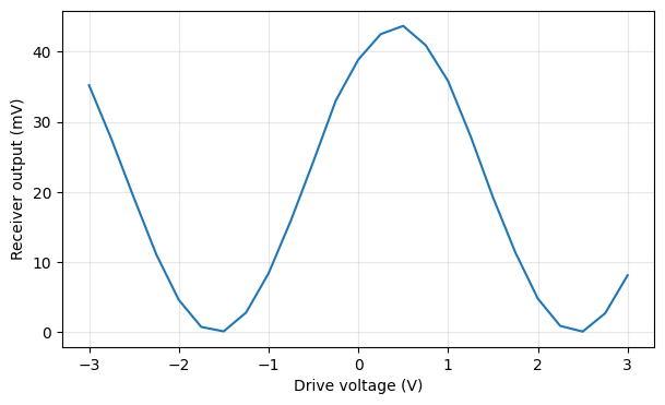
Time-domain simulation: NRZ eye diagram

Now the full 50 Gb/s test. Every model in the circuit provides a time-domain counterpart: analytic models step directly, and stored S-parameter data (like the Y splitter’s FDTD result) is automatically fitted with a pole-residue model over fit_frequencies. The laser and the two drive sources run on their own, so we simply step the circuit and record the receiver.

Each source swings between 0 and \(V_\pi/2\), and because the patterns are complementary the differential drive alternates between \(+V_\pi/2\) and \(-V_\pi/2\): exactly the null-to-maximum span we just measured.

# Put the data back on the sources after the DC sweep left them at fixed offsets
source_a.update(amplitude=drive, offset=0)
source_b.update(amplitude=drive, offset=0)

time_stepper = link.setup_time_stepper(
    time_step=time_step,
    carrier_frequency=f0,
    time_stepper_kwargs={"frequencies": fit_frequencies},
    show_progress=False,
)

result = time_stepper.step(steps=num_bits * steps_per_bit, time_step=time_step)

# The receiver output is an electrical wave in sqrt(W): sqrt(z0) turns it into volts
rx = np.real(result["RX_OUT@0"]) * np.sqrt(z0)
time = result.times

fig, (ax1, ax2) = plt.subplots(1, 2, figsize=(11, 4), tight_layout=True)

# waveform: first 16 bits
n_show = 16 * steps_per_bit
ax1.plot(time[:n_show] * 1e9, rx[:n_show] * 1e3)
ax1.set(xlabel="Time (ns)", ylabel="Receiver output (mV)", title="Received signal")
ax1.grid(True, alpha=0.3)

# Eye diagram: overlay every 2-bit window on top of the others. The first bits
# are still settling, so skip them.
skip = 8 * steps_per_bit
folded = rx[skip:]
eye_time = np.arange(steps_per_bit * 2) * time_step * 1e12  # in ps
for k in range(len(folded) // steps_per_bit - 2):
    segment = folded[k * steps_per_bit : (k + 2) * steps_per_bit]
    ax2.plot(eye_time, segment * 1e3, color="teal", alpha=0.15, lw=0.8)
ax2.set(
    xlabel="Time (ps)",
    ylabel="Receiver output (mV)",
    title=f"{bit_rate * 1e-9:g} Gb/s NRZ eye diagram",
)
ax2.grid(True, alpha=0.3)

plt.show()

Progress: 20480/20480

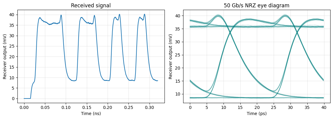
A wide-open NRZ eye with full extinction: the push-pull drive swings the interferometer between its maximum and its null, and the receiver recovers clean levels.

Want to learn more?

• Editing these components in the GUI. Everything here can be pushed to a PhotonForge project and opened in Photonic Canvas, where a teammate can change a parameter and re-run without writing Python. The PDA guide covers projects, versioning, and sharing.

• For an advanced, system-level example, follow the 800G datacom transmitter chip tutorial: it builds a complete 4-channel WDM transmitter, filters, modulators, bias calibration, and full-wave verification, step by step.

• The Mach-Zehnder modulator guide explores modulator compact models in depth: chirp, dual drive, and bandwidth effects.

• The MZM example builds a full silicon PN-depletion modulator from physical simulations.

• Browse the example library for complete transmitter and system designs.