Integrator

Accumulation is as fundamental as differentiation: a photodiode current integrated over a gate is a collected charge, the I term of a PID controller accumulates the error history, and a ramp generator is nothing but an integrator with a reset. The abstract integrator provides the running integral of an electrical signal, based on the IntegralTimeStepper:

\[y_k = y_{k-1} + s \, x_k \, \Delta t,\]

with the scaling factor \(s\) given in \(\mathrm{s}^{-1}\), so the output is \(s \int V \, dt\) and a scale near the inverse of the signal time scale keeps the output amplitude comparable to the input. Around this accumulator the stepper offers the machinery of a practical integrator:

• limits clamp the output between a lower and an upper rail,

• port E1 is an edge-triggered reset that returns the output to start_value, with reset_trigger selecting rising, falling, or both edges and reset_tolerance setting the minimum step that counts as an edge,

• the input is E0 and the output is E2.

This guide integrates a pulse, builds a sawtooth generator from the reset feature, and closes with a pulse energy meter combining optical and electrical components.

Setup

import matplotlib.pyplot as plt
import numpy as np
from scipy.special import erf
import photonforge as pf
import photonforge.abstract as pfa

viewer = pf.live_viewer.LiveViewer()

LiveViewer started at http://localhost:60054

tech = pf.basic_technology()
pf.config.default_technology = tech

f0 = pf.C_0 / 1.55
time_step = 1e-12
z0 = 50.0  # impedance of the virtual electrical ports

Integrating a Pulse

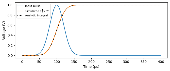
The running integral of a Gaussian pulse is the error-function step, plotted below for reference:

\[y(t) = s \int_{-\infty}^{t} V_\mathrm{pk} \, e^{-(t' - t_0)^2 / 2 \sigma^2} \, dt' = \frac{V_\mathrm{pk}}{2} \left[ 1 + \mathrm{erf} \left( \frac{t - t_0}{\sqrt{2} \sigma} \right) \right] \quad \text{for} \quad s = \frac{1}{\sqrt{2 \pi} \, \sigma}.\]

That choice of scale makes the plateau equal to the pulse peak: the output settles at \(s\) times the pulse area. The pulse is injected directly at E0 and the integral read at E2.

sigma = 20e-12  # pulse width (s)
v_pk = 1.0  # pulse peak (V)
t0 = 100e-12

num_steps = 400
t = np.arange(num_steps) * time_step
pulse = v_pk / np.sqrt(z0) * np.exp(-((t - t0) ** 2) / (2 * sigma**2))

# Scale 1 / (sqrt(2 pi) sigma) makes the output plateau at the pulse peak value
integrator = pfa.integrator(scale=1 / (np.sqrt(2 * np.pi) * sigma))
time_stepper = integrator.setup_time_stepper(
    time_step=time_step, carrier_frequency=f0, show_progress=False
)
out = time_stepper.step(
    inputs=pf.TimeSeries({"E0@0": pulse}, time_step), show_progress=False
)
integral = np.real(out["E2@0"]) * np.sqrt(z0)

analytic = v_pk / 2 * (1 + erf((t - t0) / (np.sqrt(2) * sigma)))

fig, ax = plt.subplots(figsize=(7, 3), tight_layout=True)
ax.plot(t * 1e12, pulse * np.sqrt(z0), label="Input pulse")
ax.plot(t * 1e12, integral, label="Simulated $s \\int V \\, dt$")
ax.plot(t * 1e12, analytic, "k:", label="Analytic integral")
ax.set(xlabel="Time (ps)", ylabel="Voltage (V)")
_ = ax.legend(fontsize=8)

Reset and Limits

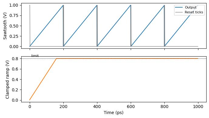
A constant input turns the integrator into a ramp generator, and the two remaining features shape that ramp. Feeding narrow ticks to the reset port E1 restarts the ramp on every rising edge, producing the classic sawtooth of a function generator. Setting limits instead clamps the accumulation at a rail, like a capacitor charged against a supply: the ramp flattens when it reaches the limit and resumes only if the input changes sign.

num_steps = 1000
t = np.arange(num_steps) * time_step
drive = 0.5 / np.sqrt(z0) * np.ones(num_steps)  # constant 0.5 V input

# Sawtooth: narrow 1 V reset ticks every 200 ps restart the ramp on their rising edges
reset_ticks = 1.0 / np.sqrt(z0) * ((t % 200e-12) < 2e-12)
sawtooth_generator = pfa.integrator(scale=1 / 100e-12)
time_stepper = sawtooth_generator.setup_time_stepper(
    time_step=time_step, carrier_frequency=f0, show_progress=False
)
out = time_stepper.step(
    inputs=pf.TimeSeries({"E0@0": drive, "E1@0": reset_ticks}, time_step),
    show_progress=False,
)
sawtooth = np.real(out["E2@0"]) * np.sqrt(z0)

# Clamped ramp: same drive, no resets, output limited to 0.8 V
clamped_integrator = pfa.integrator(scale=1 / 100e-12, limits=(0, 0.8 / np.sqrt(z0)))
time_stepper = clamped_integrator.setup_time_stepper(
    time_step=time_step, carrier_frequency=f0, show_progress=False
)
out = time_stepper.step(
    inputs=pf.TimeSeries({"E0@0": drive}, time_step), show_progress=False
)
clamped = np.real(out["E2@0"]) * np.sqrt(z0)

fig, (ax1, ax2) = plt.subplots(2, 1, figsize=(7, 4), sharex=True, tight_layout=True)
ax1.plot(t * 1e12, sawtooth, label="Output")
ax1.plot(t * 1e12, reset_ticks * np.sqrt(z0), color="tab:gray", linewidth=1, label="Reset ticks")
ax1.set(ylabel="Sawtooth (V)")
ax1.legend(fontsize=8, loc="upper right")
ax2.plot(t * 1e12, clamped, color="tab:orange")
ax2.axhline(0.8, color="black", linestyle=":", linewidth=1)
ax2.text(10, 0.83, "limit", fontsize=8)
_ = ax2.set(xlabel="Time (ps)", ylabel="Clamped ramp (V)")

Application: a Pulse Energy Meter

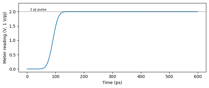
Integrating a detected photocurrent measures the energy of an optical pulse, the working principle of gated energy monitors. An optical_pulse with a known energy of 2 pJ illuminates a photodiode whose output voltage is \(V = G \, R \, P(t)\) with responsivity \(R = 1\) A/W and transimpedance gain \(G = 1\) V/A. Choosing the integrator scale as

\[s = \frac{1}{G \, R \times 1 \, \mathrm{pJ}}\]

calibrates the meter to 1 V of output per picojoule of detected energy, so the reading should settle at 2 V. The reset port is exposed as a circuit port, ready to gate consecutive measurements (and its zero drive sets the duration of the run).

responsivity = 1.0  # photodiode responsivity (A/W)
gain = 1.0  # transimpedance gain (V/A)

pulse_source = pfa.optical_pulse(energy=2e-12, width=50e-12)
photodiode = pfa.photodiode(responsivity=responsivity, gain=gain)
# Calibration: 1 V of integrator output per pJ of detected optical energy
meter = pfa.integrator(scale=1 / (gain * responsivity * 1e-12))

energy_meter = pf.Component("energy_meter")
pulse_ref = energy_meter.add_reference(pulse_source)
photodiode_ref = energy_meter.add_reference(photodiode)
meter_ref = energy_meter.add_reference(meter)
photodiode_ref.connect("P0", pulse_ref["P0"])
meter_ref.connect("E0", photodiode_ref["E0"])
energy_meter.add_port(meter_ref["E2"], "energy")
energy_meter.add_port(meter_ref["E1"], "reset")
energy_meter.add_model(pf.CircuitModel(), "Circuit")

num_steps = 600
t = np.arange(num_steps) * time_step
time_stepper = energy_meter.setup_time_stepper(
    time_step=time_step, carrier_frequency=f0, show_progress=False
)
out = time_stepper.step(
    inputs=pf.TimeSeries({"reset@0": np.zeros(num_steps)}, time_step),
    show_progress=False,
)
reading = np.real(out["energy@0"]) * np.sqrt(z0)

fig, ax = plt.subplots(figsize=(7, 3), tight_layout=True)
ax.plot(t * 1e12, reading)
ax.axhline(2.0, color="black", linestyle=":", linewidth=1)
ax.text(10, 2.04, "2 pJ pulse", fontsize=8)
ax.set(xlabel="Time (ps)", ylabel="Meter reading (V, 1 V/pJ)")
_ = ax.set_ylim(-0.1, 2.3)

Summary

• pfa.integrator accumulates \(y_k = y_{k-1} + s \, x_k \, \Delta t\): the running integral \(s \int V \, dt\) of the signal at E0 appears at E2, with the scale \(s\) in \(\mathrm{s}^{-1}\).

• The output settles at \(s\) times the pulse area for pulsed inputs, and ramps with slope \(s \, V\) for constant inputs.

• Rising (or falling, or both, per reset_trigger) edges at port E1 reset the output to start_value; a constant drive plus periodic reset ticks is a sawtooth generator.

• limits clamp the output between two rails, modeling saturation of the accumulation.

• Integrating a photodiode output measures optical pulse energy directly, with the scale providing the calibration.

• The differentiator provides the inverse operation, and the ExpressionTimeStepper covers memoryless custom math.