MMI 3 dB Coupler with EME

This example designs a 2x2 multimode interference (MMI) 3 dB coupler using the EMEModel, an eigenmode expansion (EME) solver.

MMI couplers are a textbook application of EME. Their operation relies on self-imaging: a field launched into a wide multimode region is periodically reproduced as single or multiple copies of the input as it propagates. EME is the natural method for this problem because it expands the field in the eigenmodes of each cross-section and propagates them analytically, which is far cheaper than time-stepping the whole volume with FDTD for a device that is long and dominated by propagation in a nearly uniform region.

The most valuable feature of EME for design is that the modes of a uniform section are solved only once, so the length of that section can be swept almost for free. We use exactly that capability to locate the 3 dB self-imaging length in a single simulation, and then visualize the resulting self-imaging field.

Technology

We use the built-in basic_technology, a silicon-on-insulator stack with a 220 nm device layer and a 500 nm wide single-mode strip waveguide (the "Strip" port specification).

import numpy as np
import photonforge as pf
import tidy3d as td
from matplotlib import pyplot as plt
from photonforge.live_viewer import LiveViewer

viewer = LiveViewer()

tech = pf.basic_technology()
pf.config.default_technology = tech

central_frequency = pf.C_0 / 1.55

LiveViewer started at http://localhost:52843

Parametric MMI component

The component is a wide multimode region of length length and width mmi_width, fed by two input and two output access waveguides. Linear tapers widen the 500 nm access waveguides to taper_width at the junctions with the multimode region, which reduces excitation of unwanted modes and lowers the insertion loss. The geometry is generated with stencil.mmi and a cladding envelope is added so the Strip ports are detected correctly.

The access waveguides are placed at +/- port_separation / 2. Two points matter here:

• The separation must be large enough that a port mode does not overlap the neighboring waveguide, otherwise the port mode is ill-defined. A center-to-center separation of 2 um (1 um edge-to-edge gap) is comfortable.

• For a 2x2 coupler based on general interference, an input produces two self-images, one at the input transverse position and one mirrored about the center. Placing the outputs at the same +/- port_separation / 2 therefore captures both images.

We attach an EMEModel inside the function. The EME grid divides the device along the propagation direction into cells where modes are solved: a few cells resolve each taper, and a single cell covers the uniform multimode region, where one cell is exact because the propagation there is analytic. The accuracy and cost are set by num_modes and taper_cells; we justify the defaults of 20 and 8 in the convergence study near the end. An optional add_field_monitor flag attaches a small EMEFieldMonitor, restricted to the two low-order modes and the Ey component, so the propagated field can be recovered from a single-frequency run for visualization without producing a large dataset.

@pf.parametric_component
def mmi_coupler(
    *,
    length=56.5,
    mmi_width=4.0,
    port_length=5.0,
    taper_width=1.5,
    port_separation=2.0,
    num_modes=20,
    taper_cells=8,
    add_field_monitor=False,
):
    mmi = pf.Component("MMI_2x2")

    geometry = pf.stencil.mmi(
        length=length,
        width=mmi_width,
        num_ports=(2, 2),
        port_length=port_length,
        port_width=0.5,
        tapered_width=taper_width,
        port_separation=port_separation,
    )
    mmi.add("WG_CORE", *geometry)
    mmi.add("WG_CLAD", pf.envelope(mmi, offset=1.0, trim_x_min=True, trim_x_max=True))
    mmi.add_port(mmi.detect_ports([tech.ports["Strip"]]))

    # EME cells: taper_cells per taper, a single cell for the uniform region.
    x_min = mmi.bounds()[0][0]
    mode_spec = td.EMEModeSpec(num_modes=num_modes)
    eme_grid = td.EMECompositeGrid(
        subgrids=[
            td.EMEUniformGrid(num_cells=taper_cells, mode_spec=mode_spec),
            td.EMEUniformGrid(num_cells=1, mode_spec=mode_spec),
            td.EMEUniformGrid(num_cells=taper_cells, mode_spec=mode_spec),
        ],
        subgrid_boundaries=[x_min + port_length, x_min + port_length + length],
    )

    monitors = []
    if add_field_monitor:
        # Keep the field data small: only the two low-order (even/odd) modes and
        # the Ey component are needed to reconstruct a single-port TE field.
        monitors = [
            td.EMEFieldMonitor(
                center=(0, 0, 0.11),
                size=(td.inf, td.inf, 0),
                name="field",
                num_modes=2,
                fields=["Ey"],
            )
        ]
    mmi.add_model(pf.EMEModel(eme_grid_spec=eme_grid, monitors=monitors), "EME")

    return mmi


mmi = mmi_coupler()
viewer(mmi)

The four ports are detected as P0, P1 (inputs, left) and P2, P3 (outputs, right). With a single input at P0, P2 is the bar output (same side as the input) and P3 is the cross output.

Finding the 3 dB length with an EME length sweep

The length of the uniform multimode region sets the splitting ratio. A first estimate comes from the beat length of the two lowest modes of the multimode region, L_pi = pi / (beta_0 - beta_1). For this 4 um wide region L_pi is about 39 um, and the two-fold (3 dB) self-image of general interference forms near 3 * L_pi / 2, about 59 um. This is only a starting point, so we sweep the length to locate the true 3 dB point.

Instead of rebuilding and re-simulating the device at every length, we use the native EME length sweep through the simulation_updates argument of the model. A tidy3d.EMELengthSweep scales the length of selected EME cells without re-solving the modes: only the analytic propagation phase changes. We scale only the single central cell, so every length in the sweep reuses the same modes and the whole sweep runs as one simulation.

The scale_factors array has one row per swept length and one column per EME cell. All columns are 1 except the central-cell column, which carries length / base_length.

base_length = 56.0
swept_lengths = np.linspace(20.0, 75.0, 56)

mmi_sweep = mmi_coupler(length=base_length)
eme_grid = mmi_sweep.models["EME"].eme_grid_spec

subgrids = eme_grid.subgrids
num_cells = sum(sub.num_cells for sub in subgrids)
center_cell = subgrids[0].num_cells  # index of the uniform-region cell

# Scale only the central (uniform) cell, leaving the taper cells fixed.
scale_factors = np.ones((swept_lengths.size, num_cells))
scale_factors[:, center_cell] = swept_lengths / base_length

# A dedicated model carries the length sweep so the component's own model,
# reused later for characterization, is left untouched.
sweep_model = pf.EMEModel(
    eme_grid_spec=eme_grid,
    simulation_updates={"sweep_spec": td.EMELengthSweep(scale_factors=scale_factors.tolist())},
)
eme_data = sweep_model.simulation_data(mmi_sweep, [central_frequency], show_progress=False)

13:18:07 Eastern Daylight Time Loading simulation from local cache. View cached
                               task using web UI at
                               'https://tidy3d.simulation.cloud/workbench?taskId
                               =eme-0dd18339-bcac-46c5-9f37-9130dd1829a8'.

                               Loading simulation from local cache. View cached
                               task using web UI at
                               'https://tidy3d.simulation.cloud/workbench?taskId
                               =mo-6ad24a47-f7fa-4c8e-9bf3-130edc2c35a3'.

                               Loading simulation from local cache. View cached
                               task using web UI at
                               'https://tidy3d.simulation.cloud/workbench?taskId
                               =mo-381fd269-76db-4384-93ac-ac306129976f'.

                               Loading simulation from local cache. View cached
                               task using web UI at
                               'https://tidy3d.simulation.cloud/workbench?taskId
                               =mo-cd3a6e16-2069-4af4-8688-7e005a00cfe8'.

                               Loading simulation from local cache. View cached
                               task using web UI at
                               'https://tidy3d.simulation.cloud/workbench?taskId
                               =mo-2dc47d7d-2d02-4f1f-9d2c-402a7910fc76'.

The swept scattering matrix eme_data.smatrix is expressed in the basis of the EME port modes. Because the two access waveguides are well separated, the port modes of each facet are the symmetric (even) and antisymmetric (odd) supermodes of the waveguide pair, returned as mode indices 0 and 1. A single-waveguide excitation is a balanced combination of these supermodes,

\[P_0 = \tfrac{1}{\sqrt 2}\,(\text{even} + \text{odd}), \qquad P_2 = \tfrac{1}{\sqrt 2}\,(\text{even} + \text{odd}), \qquad P_3 = \tfrac{1}{\sqrt 2}\,(\text{even} - \text{odd}),\]

so the bar and cross transmissions for a P0 input follow from the four supermode-to-supermode terms of S21. This even/odd decomposition is the standard way to read physical-port results from a 2x2 MMI EME simulation (see the Tidy3D community example Cascaded 2x2 MMI array); it reproduces what the high-level s_matrix call computes internally. We wrap it in a small helper so the same step serves both the length sweep here and the mode-convergence sweep later.

def bar_cross(s21):
    """Physical bar and cross power for a P0 input, from the EME supermode
    S21 block. The last two axes of `s21` are (mode_out, mode_in)."""
    ee, eo = s21[..., 0, 0], s21[..., 0, 1]
    oe, oo = s21[..., 1, 0], s21[..., 1, 1]
    bar = np.abs(0.5 * (ee + eo + oe + oo)) ** 2
    cross = np.abs(0.5 * (ee + eo - oe - oo)) ** 2
    return bar, cross


t_bar, t_cross = bar_cross(eme_data.smatrix.S21.isel(f=0).values)

# 3 dB length: the most balanced split among low-loss, long-device solutions.
candidate = (swept_lengths > 45.0) & (t_bar + t_cross > 0.85)
best = np.argmin(np.where(candidate, np.abs(t_bar - t_cross), np.inf))
optimal_length = swept_lengths[best]
print(f"3 dB length: {optimal_length:.1f} um")
print(f"  bar = {t_bar[best]:.3f}, cross = {t_cross[best]:.3f}, "
      f"total = {t_bar[best] + t_cross[best]:.3f}")

3 dB length: 57.0 um
  bar = 0.486, cross = 0.488, total = 0.974

fig, ax = plt.subplots(figsize=(7, 4), tight_layout=True)
ax.plot(swept_lengths, t_bar, label="bar (P0 to P2)")
ax.plot(swept_lengths, t_cross, label="cross (P0 to P3)")
ax.axvline(optimal_length, color="k", ls="--", lw=1)
ax.set_xlabel("Multimode region length (um)")
ax.set_ylabel("Transmitted power")
ax.set_title("EME length sweep (single simulation)")
ax.legend()
ax.grid(True, alpha=0.3)
plt.show()

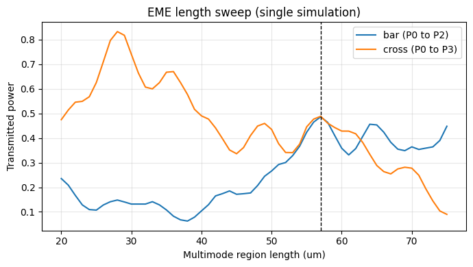
The bar and cross curves cross near the predicted length, where the input power splits equally between the two outputs. Around 28 um the device acts instead as a cross-over (the single mirrored image), and the 3 dB point sits at roughly twice that length, as expected for two-fold imaging.

Convergence

The cost and accuracy of the model are controlled by the number of modes kept in each cell and the number of cells resolving the tapers. We verify both at the design length. The mode count is swept in a single simulation with tidy3d.EMEModeSweep, which reuses one mode solve and repeats only the propagation with fewer modes. The taper-cell count changes the mode-solving grid, so it needs a separate build per value.

# Mode-count convergence in a single simulation with EMEModeSweep.
mode_counts = [4, 8, 12, 16, 20, 24]
conv = mmi_coupler(length=optimal_length, num_modes=max(mode_counts))
mode_sweep_model = pf.EMEModel(
    eme_grid_spec=conv.models["EME"].eme_grid_spec,
    simulation_updates={"sweep_spec": td.EMEModeSweep(num_modes=mode_counts)},
)
mode_s21 = mode_sweep_model.simulation_data(
    conv, [central_frequency], show_progress=False
).smatrix.S21.isel(f=0).values
mode_bar, mode_cross = bar_cross(mode_s21)

# Taper-cell convergence: one build per value (the mode grid changes).
cell_counts = [2, 4, 8, 12]
cell_total = []
for n in cell_counts:
    s = mmi_coupler(length=optimal_length, taper_cells=n).s_matrix(
        [central_frequency], model_kwargs={"inputs": ["P0"]}
    )
    cell_total.append(np.abs(s["P0@0", "P2@0"][0]) ** 2 + np.abs(s["P0@0", "P3@0"][0]) ** 2)

fig, (ax1, ax2) = plt.subplots(1, 2, figsize=(9, 3.2), tight_layout=True)
ax1.plot(mode_counts, mode_bar + mode_cross, "o-")
ax1.set_xlabel("Number of modes")
ax1.set_ylabel("Total transmission")
ax1.set_title("Mode convergence (EMEModeSweep)")
ax1.grid(True, alpha=0.3)
ax2.plot(cell_counts, cell_total, "s-")
ax2.set_xlabel("Cells per taper")
ax2.set_ylabel("Total transmission")
ax2.set_title("Taper-cell convergence")
ax2.grid(True, alpha=0.3)
plt.show()

Uploading task 'EME…'
Uploading task 'Mode-Stripwaveguide…'
Uploading task 'Mode-Stripwaveguide…'
Uploading task 'Mode-Stripwaveguide…'
Uploading task 'Mode-Stripwaveguide…'
Starting task 'Mode-Stripwaveguide': https://tidy3d.simulation.cloud/workbench?taskId=mo-154abaf1-960d-4b59-9487-ec0438c7c5f0
Starting task 'Mode-Stripwaveguide': https://tidy3d.simulation.cloud/workbench?taskId=mo-8ca028ea-5cd9-4110-95d4-7534cb4684ee
Starting task 'Mode-Stripwaveguide': https://tidy3d.simulation.cloud/workbench?taskId=mo-2459b32c-71be-4bfb-955b-f0d9ebe50e86
Starting task 'Mode-Stripwaveguide': https://tidy3d.simulation.cloud/workbench?taskId=mo-f31ee02d-9ac4-485e-95f5-7bfc1c131f04
Downloading data from 'Mode-Stripwaveguide'…
Downloading data from 'Mode-Stripwaveguide'…
Downloading data from 'Mode-Stripwaveguide'…
Downloading data from 'Mode-Stripwaveguide'…
Starting task 'EME': https://tidy3d.simulation.cloud/workbench?taskId=eme-8ad9beca-424c-4243-af2f-57ddca189d99
Downloading data from 'EME'…
Uploading task 'EME…'
Starting task 'EME': https://tidy3d.simulation.cloud/workbench?taskId=eme-319fdc37-4cec-423c-aa8f-f29064243fb4
Downloading data from 'EME'…
Uploading task 'EME…'
Starting task 'EME': https://tidy3d.simulation.cloud/workbench?taskId=eme-e984efca-c463-43ce-a244-35ba9d85cc41
Downloading data from 'EME'…
Uploading task 'EME…'
Starting task 'EME': https://tidy3d.simulation.cloud/workbench?taskId=eme-7ad36537-d74b-4cfe-a2d8-04bf05b18da7
Downloading data from 'EME'…
Uploading task 'EME…'
Starting task 'EME': https://tidy3d.simulation.cloud/workbench?taskId=eme-f1c24841-ea0b-4250-843f-ce392e2384e2
Downloading data from 'EME'…

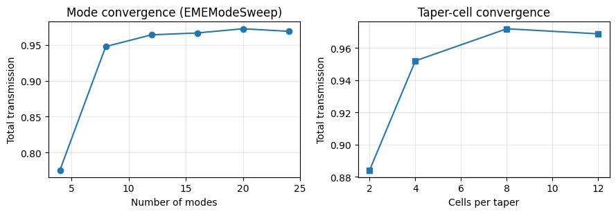
Both curves flatten by num_modes = 20 and taper_cells = 8, confirming the defaults are converged while keeping the simulation small.

Visualizing the self-imaging

We recover the field from a small dedicated run at the center wavelength: the coupler is rebuilt with add_field_monitor=True, and its monitor stores only the two low-order modes and the Ey component, so a single frequency keeps the dataset small. The field for a single P0 input follows from the same even/odd combination used for the scattering matrix.

field_coupler = mmi_coupler(length=optimal_length, add_field_monitor=True)
field_data = field_coupler.models["EME"].simulation_data(
    field_coupler, [central_frequency], show_progress=False
)["field"]

ey = field_data.Ey.isel(eme_port_index=0, sweep_index=0, z=0, f=0)
p0_ey = (ey.isel(mode_index=0).values + ey.isel(mode_index=1).values) / np.sqrt(2)
intensity = np.nan_to_num(np.abs(p0_ey) ** 2)

x = field_data.Ey.x.values
y = field_data.Ey.y.values

fig, ax = plt.subplots()

ax.pcolormesh(x, y, intensity.T / intensity.max(), cmap="magma_r", shading="auto")

# Scale the y-direction by a factor of 8
ax.set_aspect(5)

ax.set_ylim(-2.5, 2.5)
ax.set_xlabel("x (um)")
ax.set_ylabel("y (um)")
ax.set_title("Self-imaging field intensity for a P0 input")
plt.show()

Uploading task 'EME…'
Starting task 'EME': https://tidy3d.simulation.cloud/workbench?taskId=eme-dd5c80ce-1cf8-4578-a406-3e41e816a743
Downloading data from 'EME'…

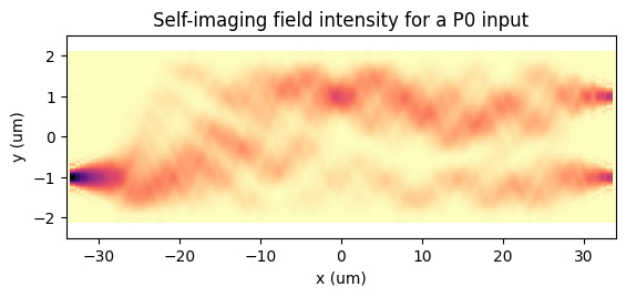
Light launched into the lower input refocuses into two equal images at the output facet, which is the self-imaging that produces the balanced 3 dB split.

At the 3 dB length the input power splits almost equally between the two outputs with low excess loss, as the length sweep reports and the self-imaging field confirms. As a 2x2 MMI, the coupler also imparts the characteristic 90 degree phase between its bar and cross outputs, the signature of a 3 dB hybrid. The design was cross-checked against a full 3D FDTD simulation (Tidy3DModel), which reproduces the same balanced split and quadrature phase.

Reference

1. Soldano, Lucas B., and Erik C. M. Pennings. “Optical multi-mode interference devices based on self-imaging: principles and applications.” Journal of Lightwave Technology 1995 13 (4), 615-627, doi: 10.1109/50.372474.

2. Tidy3D community example, “Cascaded 2x2 MMI array: EME simulation and S-parameter extraction,” flexcompute.com/tidy3d/community/notebooks/MMIEME.