Efficient simulation of a large, high-\(Q\) micro-ring resonator

High-\(Q\) micro-ring resonators are central to many integrated-photonic systems, from narrow-linewidth lasers and filters to chip-scale atomic clocks. They are also among the most expensive devices to model with full-wave FDTD: a single high-\(Q\) ring can be hundreds of micrometres across, and its photon lifetime spans millions of optical cycles, so a direct time-domain simulation of the whole device is effectively intractable on both memory and run-time grounds.

This example shows how to simulate such a ring efficiently in PhotonForge by spending FDTD only where it is physically required, the bus-to-ring coupling gap, and describing every other part of the ring with fast analytic models. The coupling gap is the one place where the two waveguides interact in a way no closed-form model captures; the straight and curved sections are well described analytically once their effective index, group index, and propagation loss are known. We compute the gap response once with FDTD, cache it, and then assemble and sweep the full ring at essentially zero additional cost.

To keep the demonstration concrete we benchmark against a measured device, the 1.38-million-\(Q\) Silicon nitride micro-ring at 780 nm reported by M. Sinclair et al. [1]. The workflow itself is general and applies to any large ring.

The steps are:

• parametric.ring_coupler builds a realistic bus-ring coupling layout.

• DirectionalCouplerCircuitModel decomposes the coupler into a central coupling region plus four arms; the coupling region is solved with FDTD (Tidy3DModel) and the arms with AnalyticWaveguideModel, so the arms cost nothing.

• We run the coupling region once over a broad band and cache it as a DataModel; caching the coupling region alone (not the whole coupler) keeps the cache valid on a coarse grid, so the dense sub-pm sweeps needed to resolve a \(Q\sim10^6\) line then need no further FDTD.

• A single 180-degree bend closes the ring analytically, and a top-level CircuitModel assembles everything.

Bend loss is negligible at this radius, so we account only for propagation loss, which we derive from the measured \(Q\) and extinction ratio rather than assume.

Reference

1. Sinclair, Martin, et al. “1.4 million Q factor Si3N4 micro-ring resonator at 780 nm wavelength for chip-scale atomic systems.” Optics express 2020 28 (3), 4010-4020, doi: 10.1364/OE.381224.

import matplotlib.pyplot as plt
import numpy as np
import photonforge as pf
import tidy3d as td
from scipy.optimize import curve_fit
from scipy.signal import find_peaks

# Interactive layout viewer.
viewer = pf.live_viewer.LiveViewer()

LiveViewer started at http://localhost:49860

Device parameters

The numbers below come from the paper and serve as targets and as a reference for comparison.

Quantity	Value	Source
Wavelength	780 nm (Rb D2 line, 780.24 nm)	Abstract
Si\(_3\)N\(_4\) core	200 nm thick \(\times\) 1100 nm wide	Fig. 5(a)
Bottom oxide / top cladding	4 µm / 900 nm SiO\(_2\)	text
\(n\)(Si\(_3\)N\(_4\)) / \(n\)(SiO\(_2\)) @ 780 nm	1.9973 / 1.454	Fig. 1(a)
Ring diameter	600 µm (radius 300 µm)	Table 1
Loaded \(Q\)	\((1.38\pm0.04)\times10^6\)	Table 2
Extinction ratio	46.8 %	Table 2
FWHM	\(570\pm20\) fm	Table 2
FSR	\(99\pm3\) pm (\(49\pm1\) GHz)	Fig. 5(b)
Power coupling	~0.4 %	text

We treat the loaded \(Q\) and the extinction ratio as the primary measured inputs and derive the propagation loss and the coupling from them below.

# --- Material and geometry ---
wl0 = 0.780  # um  design wavelength
f0 = pf.C_0 / wl0  # Hz  (pf.C_0 is in um/s)
n_core = 1.9973  # Si3N4 at 780 nm
n_clad = 1.454  # SiO2 at 780 nm
core_t, core_w = 0.200, 1.100
box_t, clad_t = 4.0, 0.900
ring_radius = 300.0  # um  (600 um diameter)
L_um = 2 * np.pi * ring_radius  # intended round-trip length

# Frequency grid for the FDTD (broad band, coarse: the coupling region is spectrally smooth).
freqs_coarse = pf.C_0 / np.linspace(0.760, 0.800, 31)

# Paper values used as targets and for comparison
paper = dict(
    Q=1.38e6,
    ER_pct=46.8,
    FWHM_fm=570.0,
    FSR_GHz=49.0,
    FSR_pm=99.0,
    coupling_pct=0.4,
    lam_nm=779.9,
)
print(f"f0 = {f0:.4e} Hz,   intended round-trip length 2*pi*R = {L_um:.1f} um")

f0 = 3.8435e+14 Hz,   intended round-trip length 2*pi*R = 1885.0 um

A realistic Si\(_3\)N\(_4\) technology

basic_technology assembles a complete layer stack (core, claddings, buried oxide, substrate) and returns a single-mode Strip port that we can solve and route with. We feed it the paper’s geometry and the 780 nm refractive indices. The default substrate medium is dispersive crystalline silicon, which is outside its validity range at 780 nm and would emit warnings; since the mode sits 4 µm above it, we replace it with a constant-index medium of the same value, which is exact for our purposes and silent.

tech = pf.basic_technology(
    core_medium=td.Medium(permittivity=n_core**2),
    clad_medium=td.Medium(permittivity=n_clad**2),
    substrate_medium=td.Medium(permittivity=3.48**2),
    core_thickness=core_t,
    strip_width=core_w,
    box_thickness=box_t,
    clad_thickness=clad_t,
)
tech.name = "SiN_780nm"
pf.config.default_technology = tech
print("Port specs:", list(tech.ports))

Port specs: ['CPW', 'Rib', 'Strip']

Waveguide cross section

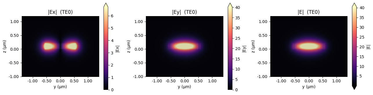
A mode solve on the Strip port gives the TE0 effective index \(n_\mathrm{eff}\), which sets the resonance positions, and the group index \(n_\mathrm{group}\), which sets the free spectral range and the conversion between finesse and \(Q\).

mode = pf.port_modes("Strip", [f0], group_index=True)
n_eff = mode.data.n_eff.isel(mode_index=0).values[0]
n_group = mode.data.n_group.isel(mode_index=0).values[0]
print(f"TE0  n_eff = {n_eff:.4f}   n_group = {n_group:.4f}")

Starting…

11:56:28 Eastern Daylight Time Loading simulation from local cache. View cached
                               task using web UI at
                               'https://tidy3d.simulation.cloud/workbench?taskId
                               =mo-99fe935d-bb31-4283-afae-6d56b3f7a12c'.

Progress: 100%
TE0  n_eff = 1.7157   n_group = 2.0020

Inspect the mode profile

Plotting the field components confirms that this is the fundamental TE mode (dominant \(E_x\), well confined in the core) before we rely on its \(n_\mathrm{eff}\) and \(n_\mathrm{group}\).

fig, axes = plt.subplots(1, 3, figsize=(13, 3.4), tight_layout=True)
for ax, comp in zip(axes, ["Ex", "Ey", "E"]):
    mode.plot_field(comp, "abs", mode_index=0, f=f0, ax=ax)
    ax.set_title(f"|{comp}|  (TE0)")
plt.show()

Propagation loss and coupling from the measured \(Q\) and ER

For an all-pass ring the through-port spectrum is set by two field quantities: the self-coupling \(t\) (with power coupling \(\kappa^2 = 1-t^2\)) and the round-trip amplitude \(a\) (the loss). The measured loaded \(Q\) and extinction ratio pin both down:

\[\text{finesse}\;\;\mathcal{F} = \frac{Q}{m},\qquad m = \frac{n_g L}{\lambda_0},\qquad \mathcal{F} = \frac{\pi\sqrt{ta}}{1-ta},\qquad \text{ER} = 1-\left(\frac{t-a}{1-ta}\right)^2 .\]

Solving for \(t\) and \(a\) gives the propagation loss (\(a\) over the round-trip length) and the power coupling \(\kappa^2\). We then confirm the values with PhotonForge’s analytic RingModel and check the coupling against the paper’s ~0.4 %.

Q_paper, ER_paper = paper["Q"], paper["ER_pct"] / 100

# Two measured numbers (Q, ER) -> two unknowns (t, a). Work through finesse first.
m = n_group * L_um / wl0  # group mode number (resonances near 780 nm)
F = Q_paper / m  # finesse = Q / m

# Invert F = pi*sqrt(ta)/(1-ta) for sqrt(ta): it is a quadratic (F/pi) y^2 + y - (F/pi) = 0.
# Keep the physical root 0 < sqrt(ta) < 1.
x = np.roots([F / np.pi, 1.0, -F / np.pi])
sqrt_ta = float(x[(x > 0) & (x < 1)][0])
ta = sqrt_ta**2

# ER fixes |t-a|: ER = 1 - ((t-a)/(1-ta))^2  ->  (t-a) = sqrt(1-ER)*(1-ta).
# With t-a and t*a known, t and a are the roots of a quadratic; pick the under-coupled branch t > a.
t_minus_a = np.sqrt(1 - ER_paper) * (1 - ta)
t_plus_a = np.sqrt(t_minus_a**2 + 4 * ta)  # since (t+a)^2 = (t-a)^2 + 4*t*a
t = (t_plus_a + t_minus_a) / 2
a = (t_plus_a - t_minus_a) / 2

kappa2 = 1 - t**2  # power coupling we must hit with the gap
# a is amplitude over the round trip (L in cm)
prop_loss_dB_cm = -20 * np.log10(a) / (L_um * 1e-4)
prop_loss = prop_loss_dB_cm / 1e4  # dB/um (AnalyticWaveguideModel units)

print(
    f"From Q = {Q_paper:.2e} and ER = {ER_paper*100:.1f}% (n_g = {n_group:.3f}, L = 2*pi*R):"
)
print(f"   round-trip amplitude a = {a:.6f}   self-coupling t = {t:.6f}")
print(f"   implied propagation loss = {prop_loss_dB_cm:.3f} dB/cm")
print(
    f"   required power coupling   = {kappa2*100:.3f} %   (paper ~{paper['coupling_pct']}% "
    f"-> ratio {kappa2*100/paper['coupling_pct']:.2f})"
)

From Q = 1.38e+06 and ER = 46.8% (n_g = 2.002, L = 2*pi*R):
   round-trip amplitude a = 0.990521   self-coupling t = 0.998511
   implied propagation loss = 0.439 dB/cm
   required power coupling   = 0.298 %   (paper ~0.4% -> ratio 0.74)

# Verify the derived (loss, coupling) reproduce the paper's Q and ER with the analytic RingModel.
def lorentz(f, fc, g, A, B):
    return B - A / (1 + ((f - fc) / g) ** 2)


ring_check = pf.RingModel(
    kappa1=np.sqrt(kappa2),
    n_eff=n_eff,
    length=L_um,
    propagation_loss=prop_loss,
    n_group=n_group,
    reference_frequency=f0,
)
bb = ring_check.black_box_component(port_spec="Strip")
pk = tuple(f"{p}@0" for p in sorted(bb.ports))

# The resonance need not sit exactly at 780 nm, so locate one within an FSR, then fit it.
FSR_chk = pf.C_0 / (n_group * L_um)
fscan = np.linspace(f0 - 0.6 * FSR_chk, f0 + 0.6 * FSR_chk, 40000)
fr0 = fscan[np.argmin(np.abs(bb.s_matrix(fscan)[pk]) ** 2)]
ffit = np.linspace(fr0 - 3e9, fr0 + 3e9, 8000)
Tfit = np.abs(bb.s_matrix(ffit)[pk]) ** 2
pp, _ = curve_fit(
    lorentz,
    ffit,
    Tfit,
    p0=[ffit[np.argmin(Tfit)], 1e8, Tfit.max() - Tfit.min(), Tfit.max()],
    maxfev=40000,
)
print(
    f"RingModel check:  Q = {pp[0]/(2*abs(pp[1])):.3e} (target {Q_paper:.2e}),"
    f"  ER = {pp[2]/pp[3]*100:.1f}% (target {ER_paper*100:.1f}%)"
)

RingModel check:  Q = 1.380e+06 (target 1.38e+06),  ER = 46.8% (target 46.8%)

The coupler: the only FDTD, with analytic arms

This is the heart of the method. DirectionalCouplerCircuitModel (DCCM) takes the bus-ring coupler layout and splits it into five pieces: a central coupling region, where the bus and ring waveguides run close enough to exchange power, and four arms that carry light from that region out to the four ports. We give the coupling region a Tidy3DModel, so it is solved with full-wave FDTD, and we give every arm an AnalyticWaveguideModel, so the long curved sections cost nothing in FDTD. Because the coupling region is only tens of micrometres across, this is the only expensive simulation in the whole notebook.

The coupling region is mirror-symmetric in \(x\), so we pass port_symmetries to halve the number of FDTD runs from four to two.

make_coupler is a @pf.parametric_component: it takes the gap and a coupling-region model and returns the assembled ring_coupler. We will call it twice: with an FDTD model during the gap sweep, and with a cached DataModel for the final ring.

bus_length = 50.0  # um


def analytic_wg():
    return pf.AnalyticWaveguideModel(
        n_eff=n_eff, n_group=n_group, propagation_loss=prop_loss, reference_frequency=f0
    )


def fdtd_coupling_model(verbose=True):
    "FDTD model for the coupling region; port_symmetries halve the runs from 4 to 2."
    return pf.Tidy3DModel(
        port_symmetries=[("P2", "P3", "P0", "P1")], grid_spec=10, verbose=verbose
    )


@pf.parametric_component
def make_coupler(*, gap, coupling_region_model, name="ring_coupler"):
    cd = core_w + gap
    dc = pf.DirectionalCouplerCircuitModel(
        coupling_region_model=coupling_region_model,
        arms_model=analytic_wg(),
    )
    return pf.parametric.ring_coupler(
        port_spec="Strip",
        coupling_distance=cd,
        radius=ring_radius,
        bus_length=bus_length,
        coupling_length=0.0,
        model=dc,
        name=name,
    )


def get_coupling_region(coupler):
    "Pull out the bare 4-port coupling-region sub-component from a built coupler."
    # get_circuit() returns the decomposed coupler (1 coupling region + 4 arms). The coupling
    # region is the only reference with 4 ports; each arm has just 2.
    dc = coupler.active_model
    return next(
        r.component
        for r in dc.get_circuit(coupler).references
        if len(r.component.ports) == 4
    )


# 780 nm sits at the middle of freqs_coarse, so kappa^2 at f0 = |S(P3<-P0)|^2 at the center index.
f0_idx = len(freqs_coarse) // 2

Finding the gap with a small FDTD sweep

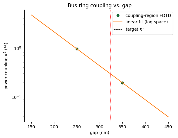
The bus-ring gap sets \(\kappa^2\). The power coupling falls off roughly exponentially with the gap, because the evanescent field of each waveguide decays exponentially into the gap and the coupling is governed by the overlap of those decaying tails. So \(\log_{10}(\kappa^2)\) is close to linear in the gap; a straight line through two swept gaps lets us solve for the gap that hits the target \(\kappa^2\).

For each swept gap we pull out the bare coupling-region sub-component and run it directly with s_matrix(freqs_coarse, model_kwargs={"inputs": ["P0"]}). This is one FDTD per gap: only the P0 excitation is needed, and the analytic arms need no simulation. Going through the full coupler instead would launch two FDTD runs per gap, because the circuit solver needs the complete coupling-region matrix to route signals.

Cost: 2 sweep points times 1 FDTD each, at roughly 2.0 FlexCredits per simulation with grid_spec=10.

# 2 single-input FDTD runs on the coupling region
sweep_gaps = np.array([0.25, 0.35])

k2_meas = []
for g in sweep_gaps:
    coupler_g = make_coupler(gap=g, coupling_region_model=fdtd_coupling_model())
    cr_g = get_coupling_region(coupler_g)  # bare coupling region
    # 1 FDTD per gap (P0 only)
    S_cr = cr_g.s_matrix(freqs_coarse, model_kwargs={"inputs": ["P0"]})
    # kappa^2 = |S(P3<-P0)|^2
    k2_meas.append(np.abs(S_cr[("P0@0", "P3@0")][f0_idx]) ** 2)
    print(f"   gap = {g*1e3:.0f} nm  ->  kappa^2 = {k2_meas[-1]*100:.4f} %")

# Linear fit of log10(kappa^2) vs gap: exact through the two points. Solve for the target kappa^2.
p_fit = np.poly1d(np.polyfit(sweep_gaps, np.log10(k2_meas), 1))
gap = float((p_fit - np.log10(kappa2)).roots[0])
print(f"\nTarget kappa^2 = {kappa2*100:.3f} %  ->  selected gap = {gap*1e3:.0f} nm")

fig, ax = plt.subplots()
ax.semilogy(
    sweep_gaps * 1e3, np.array(k2_meas) * 100, "o", label="coupling-region FDTD"
)
gg = np.linspace(0.15, 0.45, 100)
ax.semilogy(gg * 1e3, 10 ** p_fit(gg) * 100, "-", label="linear fit (log space)")
ax.axhline(kappa2 * 100, ls="--", c="k", lw=0.8, label="target $\\kappa^2$")
ax.axvline(gap * 1e3, ls=":", c="r", lw=0.8)
ax.set_xlabel("gap (nm)")
ax.set_ylabel("power coupling $\\kappa^2$ (%)")
ax.set_title("Bus-ring coupling vs. gap")
ax.legend()
plt.show()

11:56:31 Eastern Daylight Time Loading simulation from local cache. View cached
                               task using web UI at
                               'https://tidy3d.simulation.cloud/workbench?taskId
                               =fdve-5ac90b39-290e-43eb-807f-8b4e0a5128e4'.

   gap = 250 nm  ->  kappa^2 = 0.9577 %

11:56:32 Eastern Daylight Time Loading simulation from local cache. View cached
                               task using web UI at
                               'https://tidy3d.simulation.cloud/workbench?taskId
                               =fdve-6fe54337-d336-49a2-b114-65b0c8ccbe03'.

   gap = 350 nm  ->  kappa^2 = 0.1943 %

Target kappa^2 = 0.298 %  ->  selected gap = 323 nm

The coupling-region FDTD, cached

Now we run the one real FDTD, on the coupling region at the selected gap, over the broad band, and cache the result as a DataModel to reuse for every ring sweep.

One detail is essential: we cache only the coupling region, not the whole coupler. The full coupler also contains the long ring-side arms, whose phase winds very rapidly with frequency; sampling that on the coarse freqs_coarse grid and interpolating it would alias badly, giving a wrong FSR and washed-out resonances. The coupling region on its own is spectrally smooth, so the coarse grid captures it faithfully, while the arms stay fully analytic and their fast phase is evaluated exactly at every frequency, never interpolated. This is what lets the cache stay coarse. (Resolving a \(Q\sim10^6\) line needs a grid finer than about 1 MHz, tens of thousands of points across one FSR; caching avoids re-running FDTD, and its port mode solves, at every one of those points.)

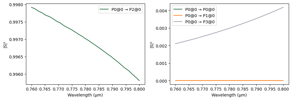
A check worth keeping. A high-\(Q\) ring has a minuscule round-trip loss budget (here about 0.08 dB), so the coupling region must be nearly lossless or the modelled \(Q\) comes out low. The cell below prints its excess loss, how much input power the 4-port S-matrix fails to conserve, taken as the worst case over all input ports. We use the worst case rather than just the bus input because the cavity circulates through the ring-side ports, so that is the loss the resonator actually feels. At grid_spec=10 it is a small fraction of a percent: well below the budget, but not exactly zero, and it is the main reason the modelled \(Q\) here lands a bit under the paper value. We cache the matrix as-is and accept that small gap to keep the workflow simple; refining the mesh (grid_spec) shrinks this excess loss, and the residual \(Q\) gap, further. If the excess loss were ever comparable to the loss budget, the other standard remedy is to project the coupling-region S-matrix onto the nearest unitary (lossless) matrix before caching (via its SVD, keeping the phases and coupling ratio but forcing power conservation); we do not need that here.

# Build the coupler at the selected gap with the FDTD coupling region, then pull that region out.
coupler_fdtd = make_coupler(
    gap=gap, coupling_region_model=fdtd_coupling_model(verbose=True)
)
cr = get_coupling_region(coupler_fdtd)
viewer(coupler_fdtd)

S_cr = cr.s_matrix(freqs_coarse)  # 2 simulations (~5 FC)

# Power-conservation check at 780 nm. For each input port, 1 - (total power out over all 4 ports)
# is the coupling region's excess (numerical) loss for that excitation. The cavity circulates
# through the ring-side ports, so we report the WORST case over all inputs (not just the bus P0),
# i.e. the loss the resonator actually sees. It must stay well under the round-trip loss budget.
cr_ports = sorted(cr.ports)
excess = max(
    1
    - sum(np.abs(np.asarray(S_cr[(f"{p}@0", f"{q}@0")])[f0_idx]) ** 2 for q in cr_ports)
    for p in cr_ports
)
print(
    f"Coupling-region excess loss at 780 nm (worst input port): {excess*100:.3f} %  "
    f"(~{-10*np.log10(1 - excess):.4f} dB; round-trip loss budget is {-20*np.log10(a):.3f} dB)"
)

# Power coupling kappa^2 = |S(P3<-P0)|^2 at 780 nm.
cross = np.abs(S_cr[("P0@0", "P3@0")][f0_idx]) ** 2
print(
    f"Power coupling at 780 nm: kappa^2 = {cross*100:.3f} %  (target {kappa2*100:.3f} %)"
)
_ = pf.plot_s_matrix(S_cr, input_ports=["P0"])

11:56:33 Eastern Daylight Time Loading simulation from local cache. View cached
                               task using web UI at
                               'https://tidy3d.simulation.cloud/workbench?taskId
                               =fdve-8986b6a8-fe6f-4e90-a2d0-72d7c0c0945c'.

                               Loading simulation from local cache. View cached
                               task using web UI at
                               'https://tidy3d.simulation.cloud/workbench?taskId
                               =fdve-6030ded4-37b5-4b83-9c43-ad4141d430a0'.

Coupling-region excess loss at 780 nm (worst input port): 0.234 %  (~0.0102 dB; round-trip loss budget is 0.083 dB)
Power coupling at 780 nm: kappa^2 = 0.299 %  (target 0.298 %)

# Cache the coupling region's S-matrix directly as a DataModel; the arms stay analytic. From here on
# the coupler (and the ring) evaluate with no FDTD: the DataModel just interpolates the stored S.
# (We cache the raw S: its small excess loss is well under the budget. If it were comparable to the
#  budget, you would refine the mesh or project S onto the nearest unitary matrix first, see above.)
coupler = make_coupler(
    gap=gap,
    coupling_region_model=pf.DataModel(
        s_matrix=S_cr, interpolation_method="cubicspline"
    ),
    name="ring_coupler_cached",
)
print(
    "Coupler coupling-region model is now cached; ring sweeps below launch no further FDTD."
)

Coupler coupling-region model is now cached; ring sweeps below launch no further FDTD.

Cost: what we avoided

cb = coupler.bounds()
ring_d = 2 * ring_radius + core_w
fdtd_w = 80.0  # um, estimate of the coupling-region FDTD window
fdtd_h = cb[1][1] - cb[0][1]  # coupling-region FDTD window (y extent)
area_ratio = (ring_d * ring_d) / (fdtd_w * fdtd_h)
tau_ph = paper["Q"] / (2 * np.pi * f0)
t_rt = n_group * (L_um * 1e-6) / (pf.C_0 * 1e-6)
n_rt = tau_ph / t_rt
print(f"Coupling-region FDTD window : {fdtd_w:.0f} x {fdtd_h:.1f} um")
print(f"Full ring footprint         : {ring_d:.0f} x {ring_d:.0f} um")
print(
    f"Cross-sectional AREA ratio  : ~{area_ratio:,.0f}x more cells for a whole-ring FDTD"
)
print(
    f"Cavity photon lifetime      : {tau_ph*1e9:.2f} ns  ({n_rt:,.0f} round trips to ring down)"
)
print(
    f"Sweep FDTD (coupling region, 1 sim/gap) : {len(sweep_gaps)} x ~2.0 FC = ~{len(sweep_gaps)*2.0:.0f} FC"
)
print(f"Final coupling-region FDTD (2 sims)     : ~5 FC")
print(f"Total                                   : ~{len(sweep_gaps)*2.0 + 5:.0f} FC")

Coupling-region FDTD window : 80 x 303.0 um
Full ring footprint         : 601 x 601 um
Cross-sectional AREA ratio  : ~15x more cells for a whole-ring FDTD
Cavity photon lifetime      : 0.57 ns  (45 round trips to ring down)
Sweep FDTD (coupling region, 1 sim/gap) : 2 x ~2.0 FC = ~4 FC
Final coupling-region FDTD (2 sims)     : ~5 FC
Total                                   : ~9 FC

Closing the ring

The coupler covers the bottom half of the ring. Its ring ports P1 and P3 sit exactly 2*radius apart, so a single 180-degree bend closes the loop. The bend is analytic and carries the derived loss.

# Top half of the ring: a single 180-degree bend, analytic (no FDTD).
bend180 = pf.parametric.bend(
    port_spec="Strip", radius=ring_radius, angle=180.0, model=analytic_wg()
)

ring = pf.Component("high_q_ring")
c_ref = ring.add_reference(coupler)
b = ring.add_reference(bend180)
b.connect("P0", c_ref["P3"])
ring.add_port([c_ref["P0"], c_ref["P2"]])  # expose only bus in / through
ring.add_model(pf.CircuitModel(), "circuit")  # assemble cached + analytic
print("Exposed ring ports:", list(ring.ports))
viewer(ring)

Exposed ring ports: ['P0', 'P1']

Resonances: free spectral range and the high-\(Q\) line

The top-level CircuitModel assembles the ring spectrum from the cached coupling region and the analytic arms and bends, so dense, sub-pm sweeps are free. We first scan a couple of free spectral ranges to measure the FSR, then zoom in on the line nearest 780 nm. Detuning is shown in pm, as in the paper.

def detuning_pm(f):
    return (
        pf.C_0 / np.asarray(f) - wl0
    ) * 1e6  # wavelength detuning from 780 nm, in pm


FSR_est = pf.C_0 / (n_group * L_um)  # rough span for the wide scan
f_scan = np.linspace(f0 - 1.6 * FSR_est, f0 + 1.6 * FSR_est, 24000)
T_scan = np.abs(ring.s_matrix(f_scan)[("P0@0", "P1@0")]) ** 2

dips, _ = find_peaks(-T_scan, prominence=0.05)  # resonances are transmission minima
FSR_Hz = float(np.median(np.diff(np.sort(f_scan[dips])))) if len(dips) >= 2 else FSR_est
FSR_pm = abs(detuning_pm(f0 + FSR_Hz) - detuning_pm(f0))

fig, ax = plt.subplots(figsize=(9, 4))
ax.plot(detuning_pm(f_scan), T_scan)
ax.set_xlabel("Detuning from 780 nm (pm)")
ax.set_ylabel("Through transmission $|S_{21}|^2$")
ax.set_title(f"Broadband transmission  -  FSR = {FSR_pm:.1f} pm ({FSR_Hz/1e9:.1f} GHz)")
plt.show()
print(
    f"Measured FSR = {FSR_Hz/1e9:.1f} GHz = {FSR_pm:.1f} pm   "
    f"(paper {paper['FSR_GHz']:.0f} GHz / {paper['FSR_pm']:.0f} pm)"
)

# Resonance nearest 780 nm, to zoom into next.
f_res0 = f_scan[dips[np.argmin(np.abs(f_scan[dips] - f0))]] if len(dips) else f0

11:56:34 Eastern Daylight Time Loading simulation from local cache. View cached
                               task using web UI at
                               'https://tidy3d.simulation.cloud/workbench?taskId
                               =mo-51d83a32-4e0d-4690-afa1-3c6770958877'.

                               Loading simulation from local cache. View cached
                               task using web UI at
                               'https://tidy3d.simulation.cloud/workbench?taskId
                               =mo-1c730948-3684-4ebf-b9ca-d0251e6628cd'.

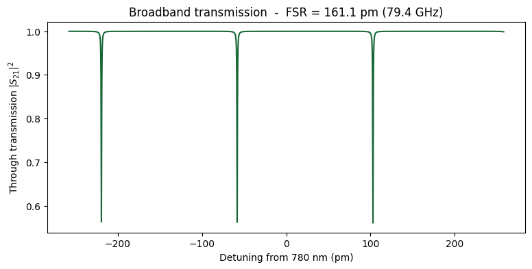
Measured FSR = 79.4 GHz = 161.1 pm   (paper 49 GHz / 99 pm)

Measured data from the paper

For a direct comparison with experiment we overlay the measured through-port trace of the resonance, digitized from Sinclair et al. Fig. 5. The raw measurement is an output power (in uW) riding on a slowly varying background, the off-resonance transmission envelope of the setup, so we divide it by a fit to that background to get a normalized transmission on the same 0-to-1 scale as the model.

# Digitized from Sinclair et al. Fig. 5. Columns: detuning from resonance (pm), output power (uW).
meas = np.array(
    [
        [-2.97, 20.25],
        [-2.79, 20.89],
        [-2.58, 21.11],
        [-2.04, 22.55],
        [-1.50, 23.76],
        [-1.17, 24.60],
        [-0.74, 24.35],
        [-0.42, 22.00],
        [-0.31, 19.91],
        [-0.19, 17.36],
        [-0.13, 15.83],
        [-0.02, 14.14],
        [0.16, 17.53],
        [0.30, 20.90],
        [0.39, 23.01],
        [0.62, 24.86],
        [1.02, 25.46],
        [1.16, 25.85],
        [1.30, 25.73],
        [1.47, 25.60],
        [1.60, 25.75],
        [1.82, 25.68],
        [1.94, 25.43],
        [2.31, 25.06],
        [2.52, 25.05],
        [2.92, 24.01],
    ]
)
# Background (off-resonance) fit from the same figure: detuning (pm), power (uW).
bg = np.array(
    [
        [-2.94, 20.20],
        [-2.13, 22.75],
        [-1.28, 24.75],
        [-0.36, 26.03],
        [0.42, 26.52],
        [1.00, 26.52],
        [1.65, 26.10],
        [2.23, 25.38],
        [2.72, 24.53],
        [2.99, 23.96],
    ]
)
det_meas = meas[:, 0]
# Normalize: divide the measured power by the background fit interpolated onto the same detunings.
T_meas = meas[:, 1] / np.interp(det_meas, bg[:, 0], bg[:, 1])

# Zoom into the resonance nearest 780 nm and fit a Lorentzian (a free analytic sweep, no FDTD).
fine_span = 4e9  # +/- 2 GHz window, wide enough for a 1.4M-Q line
f_fine = np.linspace(f_res0 - fine_span / 2, f_res0 + fine_span / 2, 8000)
T_fine = np.abs(ring.s_matrix(f_fine)[("P0@0", "P1@0")]) ** 2

# lorentz params: fc = line center, gamma = half-width at half-max, A = dip depth, B = baseline.
p0 = [f_fine[np.argmin(T_fine)], 1e8, T_fine.max() - T_fine.min(), T_fine.max()]
popt, _ = curve_fit(lorentz, f_fine, T_fine, p0=p0, maxfev=40000)
f_res, gamma, A, B = (float(v) for v in popt)

FWHM_Hz = 2 * abs(gamma)  # full width = 2 * HWHM
Q_loaded = f_res / FWHM_Hz  # loaded Q = center freq / linewidth
lam_res_nm = pf.C_0 / f_res * 1000
FWHM_fm = (wl0**2 / pf.C_0) * FWHM_Hz * 1e9  # Hz -> fm  (dlam = lam^2/c df)
ER_pct = A / B * 100  # extinction = dip depth / baseline

fig, ax = plt.subplots()
det_pm = detuning_pm(f_fine) - detuning_pm(f_res)
ax.plot(det_pm, T_fine, "-", lw=1.5, label="Circuit model")
ax.plot(det_meas, T_meas, "o", ms=5, mfc="none", label="Measured (Sinclair et al.)")
ax.set_xlabel("Detuning from resonance (pm)")
ax.set_ylabel("Normalized transmission")
ax.set_title(f"High-Q resonance at {lam_res_nm:.2f} nm   -   Q = {Q_loaded:.3e}")
ax.legend()
plt.show()

print(f"Resonance wavelength : {lam_res_nm:.2f} nm")
print(f"Loaded Q             : {Q_loaded:.3e}")
print(f"FWHM                 : {FWHM_Hz/1e6:.1f} MHz = {FWHM_fm:.0f} fm")
print(f"Extinction ratio     : {ER_pct:.1f} %")

                               Loading simulation from local cache. View cached
                               task using web UI at
                               'https://tidy3d.simulation.cloud/workbench?taskId
                               =mo-9ef68ebd-7de1-432c-8384-55cda03ba334'.

11:56:35 Eastern Daylight Time Loading simulation from local cache. View cached
                               task using web UI at
                               'https://tidy3d.simulation.cloud/workbench?taskId
                               =mo-463bae72-aa70-481c-ab51-957fc5fca3d6'.

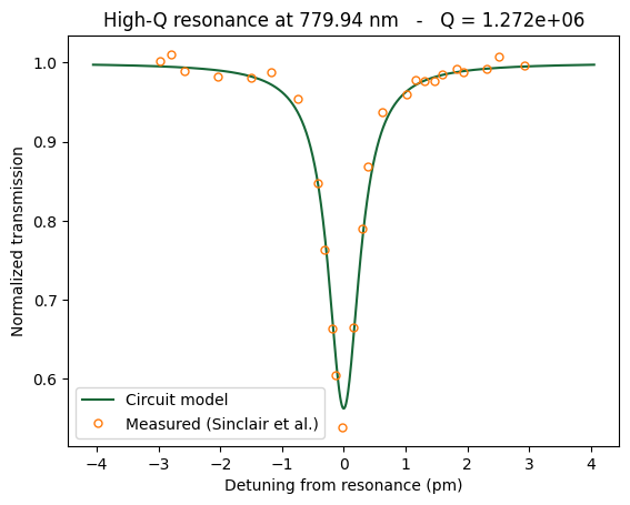
Resonance wavelength : 779.94 nm
Loaded Q             : 1.271e+06
FWHM                 : 302.4 MHz = 614 fm
Extinction ratio     : 43.9 %

Comparison with the paper

rows = [
    ("Resonance wavelength (nm)", f"{lam_res_nm:.2f}", f"{paper['lam_nm']:.1f}"),
    ("Loaded Q", f"{Q_loaded:.2e}", f"{paper['Q']:.2e}"),
    ("FWHM (fm)", f"{FWHM_fm:.0f}", f"{paper['FWHM_fm']:.0f}"),
    ("Extinction (%)", f"{ER_pct:.1f}", f"{paper['ER_pct']:.1f}"),
    ("Power coupling (%)", f"{cross*100:.2f}", f"~{paper['coupling_pct']}"),
    ("Propagation loss (dB/cm)", f"{prop_loss_dB_cm:.2f}", "derived"),
    ("FSR (pm)", f"{FSR_pm:.0f}", f"{paper['FSR_pm']:.0f}"),
]
w = max(len(r[0]) for r in rows)
print(f"{'Quantity':<{w}}   {'This model':>14}   {'Paper':>14}")
print("-" * (w + 34))
for name, sim, ref in rows:
    print(f"{name:<{w}}   {sim:>14}   {ref:>14}")

Quantity                        This model            Paper
-----------------------------------------------------------
Resonance wavelength (nm)           779.94            779.9
Loaded Q                          1.27e+06         1.38e+06
FWHM (fm)                              614              570
Extinction (%)                        43.9             46.8
Power coupling (%)                    0.30             ~0.4
Propagation loss (dB/cm)              0.44          derived
FSR (pm)                               161               99

Takeaways

• The propagation loss and coupling were derived from the measured \(Q\) and extinction ratio (loss about 0.44 dB/cm and \(\kappa^2\) about 0.3 %, both confirmed with RingModel), and the required coupling is close to the paper’s ~0.4 %. The gap was then dialed in with a tiny single-input FDTD sweep.

• DirectionalCouplerCircuitModel spends FDTD only on the coupling gap; the arms and the 180-degree bend closure are analytic with the derived loss.

• Caching the coupling region as a DataModel (not the whole coupler) is what makes every sub-pm ring sweep free while keeping the result correct. The coupling region is spectrally smooth, so a coarse cache grid captures it, whereas caching the full coupler would alias the rapidly winding ring-side arm phase. Keeping the arms analytic evaluates that fast phase exactly.

• A very high-\(Q\) ring is exquisitely sensitive to loss: its whole round-trip budget is only about 0.08 dB. The coupling region’s residual (mostly numerical) excess loss at grid_spec=10 is a small fraction of that, which leaves the modelled \(Q\) a little under the paper’s (about 1.3 versus 1.4 million). A finer mesh shrinks it; alternatively, projecting the coupling-region S-matrix onto the nearest unitary matrix before caching would remove it entirely. We keep the workflow simple and accept the small gap.

• The assembled ring closely reproduces the paper’s high-\(Q\) resonance and extinction (\(Q\) within about 10 %). The FSR follows from the simulated \(n_g\approx2.03\) (about 160 pm); the paper’s 99 pm would require a larger optical path or higher \(n_g\) than this nominal 300 µm-radius, constant-index model.