Mux/Demux Model

Wavelength-division multiplexers and demultiplexers (WDM mux/demux) are essential blocks in datacom transceivers, LiDAR, and optical computing circuits. Instead of simulating a full AWG or cascaded-filter layout, PhotonForge provides MuxDemuxModel: an analytic compact model for a single-mode WDM device with one common port and one port per channel.

Each channel is a causal band-pass filter of the Butterworth family with analytically known poles and residues. A channel centered at \(f_k\) with 3 dB bandwidth \(B_k\) and integer order \(n\) transmits

\[\lvert S_{k,\mathrm{common}}(f) \rvert^2 = \frac{10^{-IL_k/10}}{1 + \left( 2 (f - f_k) / B_k \right)^{2n}}\]

where \(IL_k\) is the insertion loss (dB). Because the response is a rational function with stable poles, its phase is the physical, causal one, and time-domain simulations consume exactly the same poles with no fitting step. The model is reciprocal, so the same component works as a multiplexer or a demultiplexer. This guide covers creating the model, shaping the passbands, per-channel parameters, channel dispersion, and temperature effects.

Setup

import matplotlib.pyplot as plt
import numpy as np
import photonforge as pf

tech = pf.basic_technology()
pf.config.default_technology = tech

wavelengths = np.linspace(1.52, 1.57, 501)
freqs = pf.C_0 / wavelengths

Creating the Model

The model can be specified with either frequencies (with bandwidth in Hz) or wavelengths (with bandwidth in μm), but not both. The number of entries defines the number of channels, and the component it is attached to must have one port per channel plus the common port.

For quick exploration we use black_box_component, which creates a component with the right number of ports without any layout. Here we build a 4-channel demux on a 10 nm grid with 200 GHz (about 1.6 nm) passbands:

channel_wavelengths = [1.53, 1.54, 1.55, 1.56]

model = pf.MuxDemuxModel(
    wavelengths=channel_wavelengths,
    bandwidth=0.0016,  # in μm, because the channels are given in wavelengths
    order=3,
    insertion_loss=0.5,
)

mux = model.black_box_component(port_spec="Strip")
mux

Port convention

When ports is not set, the model uses the component’s port names in natural order (P10 comes after P9), and the first one is the common port. In the black box above, P0 is the common port and P1 to P4 carry the channels in the order they appear in wavelengths. To attach the model to a component whose port names do not sort conveniently, pass the list explicitly, for example ports=["opt_in", "ch1", "ch2", "ch3", "ch4"], always with the common port first.

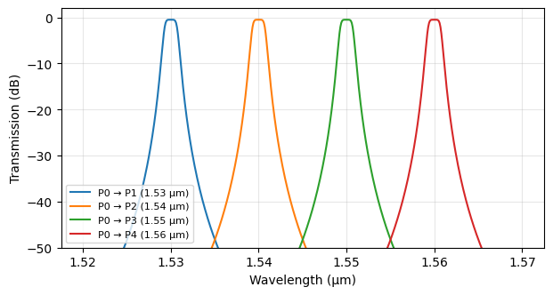
Computing the S-matrix shows one passband per channel:

s = mux.s_matrix(freqs)

fig, ax = plt.subplots(figsize=(7, 3.5))
for i, wl in enumerate(channel_wavelengths):
    t = np.abs(s[(f"P{i + 1}@0", "P0@0")]) ** 2
    ax.plot(wavelengths, 10 * np.log10(np.maximum(t, 1e-12)), label=f"P0 → P{i + 1} ({wl} μm)")
ax.set_xlabel("Wavelength (μm)")
ax.set_ylabel("Transmission (dB)")
ax.set_ylim(-50, 2)
ax.legend(fontsize=8)
ax.grid(alpha=0.3)
plt.show()

Passband Shape: Order and Bandwidth

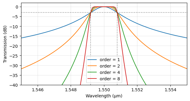
The order parameter (a positive integer) controls the passband shape. Order 1 is a single-pole Lorentzian, and higher orders produce increasingly flat-top responses with skirts falling at \(6n\) dB per octave, like higher-order cascaded filters. Regardless of order, the transmission is exactly 3 dB down at \(f_k \pm B_k/2\).

Configurations that are not passive (for example, strongly overlapping passbands with no insertion loss) are evaluated as given, with a warning instead of any silent renormalization:

fig, ax = plt.subplots(figsize=(7, 3.5))
for order in [1, 2, 4, 8]:
    single = pf.MuxDemuxModel(wavelengths=[1.55], bandwidth=0.0016, order=order)
    bb = single.black_box_component(port_spec="Strip")
    s1 = bb.s_matrix(freqs)
    t = np.abs(s1[("P1@0", "P0@0")]) ** 2
    ax.plot(wavelengths, 10 * np.log10(np.maximum(t, 1e-12)), label=f"order = {order}")
ax.axhline(-3, color="k", linestyle=":", alpha=0.5)
ax.axvline(1.55 - 0.0008, color="k", linestyle=":", alpha=0.5)
ax.axvline(1.55 + 0.0008, color="k", linestyle=":", alpha=0.5)
ax.set_xlim(1.545, 1.555)
ax.set_ylim(-40, 2)
ax.set_xlabel("Wavelength (μm)")
ax.set_ylabel("Transmission (dB)")
ax.legend()
ax.grid(alpha=0.3)
plt.show()

Per-Channel Parameters

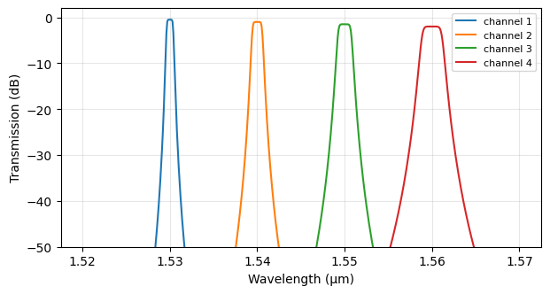
bandwidth, order, insertion_loss, and group_delay accept a sequence with one value per channel. The reflection and ports sequences need one extra entry for the common port, which comes first. Here each channel gets a different bandwidth and loss:

model_pc = pf.MuxDemuxModel(
    wavelengths=channel_wavelengths,
    bandwidth=[0.0008, 0.0012, 0.0016, 0.0024],
    insertion_loss=[0.5, 1.0, 1.5, 2.0],
    order=4,
)

mux_pc = model_pc.black_box_component(port_spec="Strip")
s_pc = mux_pc.s_matrix(freqs)

fig, ax = plt.subplots(figsize=(7, 3.5))
for i, wl in enumerate(channel_wavelengths):
    t = np.abs(s_pc[(f"P{i + 1}@0", "P0@0")]) ** 2
    ax.plot(wavelengths, 10 * np.log10(np.maximum(t, 1e-12)), label=f"channel {i + 1}")
ax.set_xlabel("Wavelength (μm)")
ax.set_ylabel("Transmission (dB)")
ax.set_ylim(-50, 2)
ax.legend(fontsize=8)
ax.grid(alpha=0.3)
plt.show()

Channel Dispersion and the Time Domain

A causal filter cannot have a flat phase: each channel carries the group delay of its Butterworth response, largest near the band edges and growing with the filter order. The group delay follows from the S-matrix phase as \(\tau_g = \frac{1}{2 \pi} \frac{\mathrm{d} \phi}{\mathrm{d} f}\) (with the sign matching PhotonForge’s \(e^{-i 2 \pi f t}\) time convention):

single = pf.MuxDemuxModel(frequencies=[pf.C_0 / 1.55], bandwidth=200e9, order=3)
bb = single.black_box_component(port_spec="Strip")

# Dense frequency grid across the passband
f_center = pf.C_0 / 1.55
f_grid = np.linspace(f_center - 300e9, f_center + 300e9, 1001)
s21 = bb.s_matrix(f_grid)[("P1@0", "P0@0")]

# Group delay from the unwrapped transmission phase
group_delay = np.gradient(np.unwrap(np.angle(s21)), f_grid) / (2 * np.pi)

fig, ax1 = plt.subplots(figsize=(7, 3.5))
ax1.plot((f_grid - f_center) / 1e9, 10 * np.log10(np.abs(s21) ** 2), color="C0")
ax1.set_xlabel("$f - f_k$ (GHz)")
ax1.set_ylabel("Transmission (dB)", color="C0")
ax1.set_ylim(-40, 2)
ax2 = ax1.twinx()
ax2.plot((f_grid - f_center) / 1e9, group_delay * 1e12, color="C1")
ax2.set_ylabel("Group delay (ps)", color="C1")
ax1.grid(alpha=0.3)
plt.show()

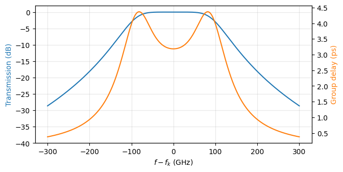
The same poles and residues drive time-domain simulations through the default SMatrixTimeStepper: there is no fitting step and no fitting error, so the time-domain response of each channel is exactly the causal counterpart of the curves above.

A constant group_delay (in seconds) adds a linear phase to each channel on top of the filter’s intrinsic dispersion, and reflection sets a constant complex reflection coefficient seen by incident fields at each port.

Temperature Sensitivity

Real WDM filters drift with temperature. Setting temperature_sensitivity shifts every channel center by \(s \cdot (T - T_\mathrm{ref})\), where the units are Hz/K when the model uses frequencies and μm/K when it uses wavelengths. A typical silicon filter drifts by roughly 0.08 nm/K:

fig, ax = plt.subplots(figsize=(7, 3.5))
for temp, style in [(293.0, "-"), (343.0, "--")]:
    model_t = pf.MuxDemuxModel(
        wavelengths=channel_wavelengths,
        bandwidth=0.0016,
        order=4,
        insertion_loss=0.5,
        temperature_sensitivity=8e-5,  # μm/K = 0.08 nm/K
        temperature=temp,
        reference_temperature=293.0,
    )
    bb_t = model_t.black_box_component(port_spec="Strip")
    s_t = bb_t.s_matrix(freqs)
    t1 = np.abs(s_t[("P1@0", "P0@0")]) ** 2
    ax.plot(wavelengths, 10 * np.log10(np.maximum(t1, 1e-12)), style, label=f"channel 1, T = {temp:.0f} K")
ax.set_xlabel("Wavelength (μm)")
ax.set_ylabel("Transmission (dB)")
ax.set_ylim(-50, 2)
ax.legend()
ax.grid(alpha=0.3)
plt.show()

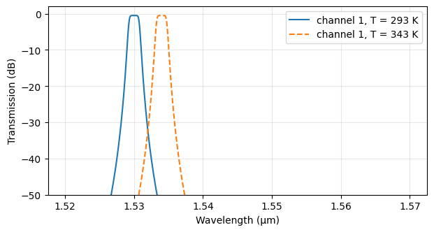
The 50 K increase shifts the channel by 4 nm, enough to move a signal into the neighboring channel, which is why athermal designs or active tuning are needed in dense WDM systems.

Abstract Component

For system-level sketches, abstract.mux_demux wraps this model in a ready-made schematic component. Its defaults follow a DWDM-style 100 GHz grid, and all model parameters can be overridden:

demux = pf.abstract.mux_demux(
    frequencies=pf.C_0 / np.array(channel_wavelengths),
    bandwidth=200e9,  # in Hz, because the channels are given in frequencies
    insertion_loss=0.5,
)
demux

The abstract component can be connected to lasers, modulators, and photodetectors from the same abstract module to assemble a full WDM link for S-matrix or time-domain analysis.

Summary

• MuxDemuxModel gives each channel a causal Butterworth passband: set centers with frequencies (Hz) or wavelengths (μm), width with bandwidth, and shape with the integer order.

• The first port (in natural order, or the first entry of ports) is the common port; the rest map to channels in order.

• Per-channel sequences are accepted for most parameters; reflection and ports take one extra leading entry for the common port. Non-passive configurations warn and are evaluated unmodified.

• The channels carry the physical dispersion of their filters, and time-domain simulations use the same analytic poles with no fitting step.

• temperature_sensitivity models thermal drift of the channel centers.

• Use black_box_component or pf.abstract.mux_demux for quick circuit-level studies before committing to a physical demux layout.