Analytic Waveguide Crossing Model

This guide covers pf.CrossingModel, which provides a compact analytic S-matrix for a 4-port waveguide crossing. It captures:

Feature	Parameter
Transmission (straight-through)	t
Cross-coupling (between arms)	x
Back-reflection	r
Dispersion (propagation phase)	propagation_length, n_eff, n_group
Frequency dependence	Interpolator for any of the above

All parameters can be complex scalars or pf.Interpolator objects for broadband characterization from measurement or FDTD simulation.

S-matrix Structure

For a crossing with ports numbered as shown below,

         P3 (top)
          |
P0 -------+------- P2
          |
         P1 (bottom)

the 4×4 S-matrix is

\[\begin{split}S = \begin{bmatrix} r & x & t & x \\ x & r & x & t \\ t & x & r & x \\ x & t & x & r \end{bmatrix} e^{j\phi}\end{split}\]

where \(t\) is the straight-through transmission (P0→P2 or P1→P3), \(x\) is the cross-coupling between arms (P0→P1), and \(r\) is the back-reflection (P0→P0).

The common phase factor \(e^{j\phi}\) models propagation through the crossing:

\[\phi = \frac{2\pi\,l_p}{c_0}\bigl[n_\mathrm{eff}\,f_0 + n_\mathrm{group}(f-f_0)\bigr]\]

where \(l_p\) is propagation_length. Setting \(l_p = 0\) (the default) removes the dispersive phase term.

import matplotlib.pyplot as plt
import numpy as np
import photonforge as pf
from photonforge.utils import C_0

pf.config.default_technology = pf.basic_technology()

C = C_0  # speed of light in µm/s
lam0 = 1.55  # µm
f0 = C / lam0

lam = np.linspace(1.50, 1.60, 1001)
freqs = C / lam

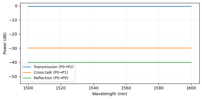
Transmission, Cross-coupling, and Reflection

Typical silicon-photonics crossing parameters at 1550 nm:

Parameter	Symbol	Typical value
Insertion loss	IL	0.2 - 0.5 dB
Cross-talk	XT	−30 to −35 dB
Return loss	RL	−40 to −50 dB

These are power quantities; CrossingModel takes the corresponding field amplitudes \(t = \sqrt{10^{-\mathrm{IL}/10}}\), etc.

IL_dB = 0.5   # insertion loss (dB)
XT_dB = -30   # cross-talk (dB)
RL_dB = -40   # return loss (dB)

# Convert to field amplitudes
t = np.sqrt(10 ** (-IL_dB / 10))
x = np.sqrt(10 ** (XT_dB / 10))
r = np.sqrt(10 ** (RL_dB / 10))
print(f"Field amplitudes:  t={t:.4f}  x={x:.5f}  r={r:.5f}")

crossing = pf.CrossingModel(t=t, x=x, r=r)
bb = crossing.black_box_component(port_spec="Strip")
s = bb.s_matrix(freqs)

fig, ax = plt.subplots(figsize=(7, 3.5))
specs = [
    ("Transmission (P0→P2)", ("P0@0", "P2@0")),
    ("Cross-talk (P0→P1)",   ("P0@0", "P1@0")),
    ("Reflection (P0→P0)",   ("P0@0", "P0@0")),
]
for label, ports in specs:
    T = np.abs(s[ports]) ** 2
    ax.plot(lam * 1e3, 10 * np.log10(T), label=label, lw=1.5)

ax.set_xlabel("Wavelength (nm)")
ax.set_ylabel("Power (dB)")
ax.set_ylim(-55, 2)
ax.legend(fontsize=9)
ax.grid(True, alpha=0.2)
fig.tight_layout()
plt.show()

Field amplitudes:  t=0.9441  x=0.03162  r=0.01000

Quick alternative: pf.abstract.crossing

pf.abstract.crossing wraps CrossingModel and returns a ready-to-use pf.Component directly - no separate model instantiation or .black_box_component() call needed. It accepts the same parameters.

comp = pf.abstract.crossing(t=t, x=x, r=r)

print("Component ports:", list(comp.ports))
comp

Component ports: ['P0', 'P1', 'P2', 'P3']

Frequency-dependent Coefficients

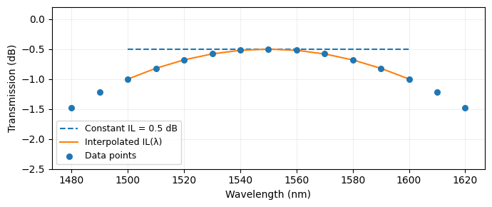
When t, x, or r are measured or simulated over a wavelength range, pass an pf.Interpolator keyed on frequency (Hz). PhotonForge interpolates the coefficients at each evaluation frequency.

Here we model an insertion loss that increases away from 1550 nm, as is typical for sub-wavelength-grating or multi-mode-interference crossing designs.

# Simulated IL vs wavelength (parabolic, minimum at 1550 nm)
lam_data = np.linspace(1.48, 1.62, 15)
IL_data = 0.5 + 2.0 * (lam_data - 1.55) ** 2 / 0.01  # dB
t_data = np.sqrt(10 ** (-IL_data / 10))
freqs_data = C / lam_data  # must pass frequencies, not wavelengths

t_interp = pf.Interpolator(freqs_data, t_data)
crossing_fd = pf.CrossingModel(t=t_interp, x=x, r=r)
bb_fd = crossing_fd.black_box_component(port_spec="Strip")
s_fd = bb_fd.s_matrix(freqs)

fig, ax = plt.subplots(figsize=(7, 3))
T_flat = np.abs(s[("P0@0", "P2@0")]) ** 2
T_fd   = np.abs(s_fd[("P0@0", "P2@0")]) ** 2
ax.plot(lam * 1e3, 10 * np.log10(T_flat), "--", label="Constant IL = 0.5 dB", lw=1.5)
ax.plot(lam * 1e3, 10 * np.log10(T_fd),         label="Interpolated IL(λ)", lw=1.5)
ax.scatter(lam_data * 1e3, -IL_data, s=30, zorder=5, label="Data points")
ax.set_xlabel("Wavelength (nm)")
ax.set_ylabel("Transmission (dB)")
ax.set_ylim(-2.5, 0.2)
ax.legend(fontsize=9)
ax.grid(True, alpha=0.2)
fig.tight_layout()
plt.show()

Dispersion

Setting propagation_length \(> 0\) adds a frequency-dependent phase to all S-matrix elements. This matters when multiple crossings are cascaded in a circuit simulation where the relative phase between parallel paths is wavelength-sensitive.

lp = 10.0   # propagation length through the crossing, µm
n_eff = 2.4
n_g   = 4.2

crossing_d = pf.CrossingModel(
    t=t, x=x, r=r,
    propagation_length=lp,
    n_eff=n_eff, n_group=n_g,
    reference_frequency=f0,
)
bb_d = crossing_d.black_box_component(port_spec="Strip")
s_d  = bb_d.s_matrix(freqs)

T21     = s[("P0@0", "P2@0")]
T21_d   = s_d[("P0@0", "P2@0")]
phi     = np.unwrap(np.angle(T21))
phi_d   = np.unwrap(np.angle(T21_d))

fig, axes = plt.subplots(1, 2, figsize=(9, 3))

axes[0].plot(lam * 1e3, phi,   "--", label="No dispersion", lw=1.5)
axes[0].plot(lam * 1e3, phi_d,       label=f"lp = {lp} µm", lw=1.5)
axes[0].set_xlabel("Wavelength (nm)")
axes[0].set_ylabel("Phase (rad)")
axes[0].set_title("Transmission phase")
axes[0].legend(fontsize=9)
axes[0].grid(True, alpha=0.2)

# Group delay: tau_g = d(phi)/d(omega)
omega = 2 * np.pi * freqs
gd   = np.gradient(phi,   omega) * 1e12  # ps
gd_d = np.gradient(phi_d, omega) * 1e12  # ps
axes[1].plot(lam * 1e3, gd,   "--", label="No dispersion", lw=1.5)
axes[1].plot(lam * 1e3, gd_d,       label=f"lp = {lp} µm", lw=1.5)
axes[1].set_xlabel("Wavelength (nm)")
axes[1].set_ylabel("Group delay (ps)")
axes[1].set_title("Group delay")
axes[1].legend(fontsize=9)
axes[1].grid(True, alpha=0.2)

fig.tight_layout()
plt.show()

gd_expected = n_g * lp / C  # s
print(f"Expected group delay: {gd_expected * 1e12:.3f} ps")
print(f"Computed  group delay: {gd_d[500]:.3f} ps")

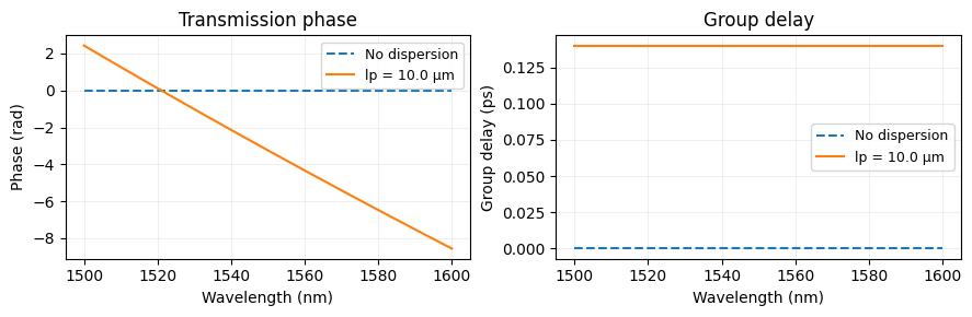
Expected group delay: 0.140 ps
Computed  group delay: 0.140 ps

pf.CrossingModel API Reference

Parameter	Type	Default	Description
t	complex | Interpolator	1.0	Straight-through field transmission
x	complex | Interpolator	0.0	Cross-coupling field coefficient
r	complex | Interpolator	0.0	Back-reflection field coefficient
propagation_length	float	0.0	Effective path length for dispersion (µm)
n_eff	complex | Interpolator	0.0	Effective index at reference frequency
n_group	float | Interpolator | None	None (→ n_eff)	Group index
reference_frequency	float | None	None (→ band center)	Taylor-expansion frequency (Hz)
ports	list[str] | None	None (→ sorted port names)	Override port ordering

All coefficients satisfy energy conservation: \(|t|^2 + |x|^2 + |r|^2 \leq 1\). Pass complex values to model amplitude and phase simultaneously.