Microring Modulator: PCell with Attached Model

The silicon microring modulator (MRM) of Yuan et al. [1] reaches 200 Gb/s per wavelength channel through a two-segment Z-shape p-n junction in the ring. The M2 routing electrode is split into two arcs around the ring; each arc drives an independent junction, and the two junctions combine optically inside the ring so that two binary drivers can produce a PAM-4 optical output.

A previous PhotonForge notebook, Two-Segment MRM, already simulates this device end-to-end. This notebook starts from the same device but with two implementation differences:

• The full layout is built as a single parametric cell (PCell) through the @pf.parametric_component decorator. The PCell draws the silicon racetrack, the slab envelope, the split M2 electrode (including the Z-junction notches), and the TiN heater all in one place, and exposes optical ports P0/P1 plus six electrical terminals (MSB±, LSB±, H±) for routing. The same PCell is reused later to build the chip-level bond-pad layout.

• The optical response is provided by PhotonForge’s built-in pf.RingModel + pf.RingTimeStepper pair calibrated directly from the paper (bus-ring power coupling κ₁, propagation loss, electro-optic slope, thermal sensitivity, MSB RC bandwidth), so no custom waveguide model is needed. The cell answers s_matrix queries directly and reproduces paper Figure 2 (FSR 5.7 nm, ER 16 dB, Q ≈ 3700, MSB tuning 16.3 pm/V, TiN heater tuning 73 pm/mW). With the paired RingTimeStepper, a CW laser, a photodiode and pf.CircuitTimeStepper, the same PCell drives a 100 Gb/s NRZ time-domain link that reproduces the MSB-only eye of paper Figure 4c. A virtual electrical DRIVE port is added on top of the layout so the time-domain solver can apply the MSB voltage waveform directly.

The two-segment architecture in the paper supports true PAM-4 from two binary drivers (one on each junction). The RingModel / RingTimeStepper pair used here lumps the optical response into a single voltage knob and therefore only captures the MSB-only case; the LSB segment is still present in the layout and is routed to its own bond pads in the chip-level section. Driving both junctions independently to recover PAM-4 would require a custom waveguide model with two voltage inputs (as in Two-Segment MRM) and is left out of this notebook.

References

1. Yuan, Yuan, et al. “A 5× 200 Gbps microring modulator silicon chip empowered by two-segment Z-shape junctions.” Nature Communications, 2024 15 (1), 918, doi: 10.1038/s41467-024-45301-3

We use the SiEPIC EBeam silicon stack as a fab-agnostic standin. Ring radius, Euler fraction and TE port specification are set as global defaults so that downstream parametric routines pick them up without being passed explicitly.

import matplotlib.pyplot as plt
import numpy as np
import photonforge as pf
import photonforge.abstract as pfa
import siepic_forge as siepic
import tidy3d as td
from matplotlib.gridspec import GridSpec
from photonforge.abstract import _virtual_port_spec
from photonforge.live_viewer import LiveViewer

viewer = LiveViewer()
# Pick the silicon EBeam PDK and pin a few defaults so we do not
# have to repeat them when building waveguides and routes.
tech = siepic.ebeam()
pf.config.default_technology = tech
pf.config.default_kwargs["radius"] = 12.0
pf.config.default_kwargs["euler_fraction"] = 0.5
pf.config.default_kwargs["port_spec"] = tech.ports["TE_1550_500"]
pf.config.svg_labels = False

08:17:51 EDT WARNING: The material-library variant 'Palik_Lossless' is          
             deprecated and maps to 'Palik_LowLoss' because it contains a tiny  
             fitted loss despite its name. Use 'Palik_NoLoss' where available   
             for a zero-loss Palik model.                                       

LiveViewer started at http://localhost:39389

The numerical values in the next cell are taken directly from the paper, with no fitting. The ring has a 12 µm radius and a 5.7 nm FSR at 1.31 µm. Propagation loss is 129 dB/cm and the bus-ring power coupling magnitude is \(\lvert\kappa_1\rvert = 0.387\), chosen so the simulated Q and extinction ratio land on the measured values. The MSB junction moves the resonance by 16.3 pm/V; converting that to a refractive index sensitivity through \(Δλ/λ = Δn_\text{eff}/n_g\) gives the ring-averaged dn_dv used by the model. The TiN heater contributes 73 pm/mW through a 1.2 K/mW thermal resistance. The 64 GHz MSB RC bandwidth from the paper’s equivalent-circuit fit goes into the time-domain stepper.

We pass the bus-ring coupling as kappa1 = 1j * 0.387 rather than just 0.387 to follow the standard directional-coupler convention: in a lossless 2×2 coupler the cross-coupled field leads the through-coupled field by a π/2 phase, so the cross-coupling coefficient is purely imaginary (\(\kappa = i\lvert\kappa\rvert\)) while the through coefficient \(\tau = \sqrt{1 - \lvert\kappa\rvert^2}\) is real positive, giving the unitary coupler matrix

\[\begin{split}\begin{bmatrix} \tau & i\kappa \\ i\kappa & \tau \end{bmatrix}\end{split}\]

with \(\tau^2 + \kappa^2 = 1\). With this convention the ring’s \(S_{21}\) minimum sits at a round-trip phase of 0 (mod 2π), so picking n_eff to place the m-th longitudinal mode at the carrier frequency lands the simulated resonance exactly on 1310 nm.

# Ring geometry
wavelength_um = 1.310
r_ring_um = 12.0
l_ring_um = 2 * np.pi * r_ring_um  # round-trip length
fsr_nm = 5.7

# Optical: group index from FSR, effective index near 1.31 um,
# propagation loss in dB/um, and bus-ring power coupling.
n_group = wavelength_um**2 / (fsr_nm * 1e-3 * l_ring_um)
n_eff_nominal = 2.4504
alpha0_dbum = 0.0129
kappa1 = 1j * 0.387

# MSB junction: convert measured d(lambda)/dV to ring-averaged dn/dV.
dlambda_dv_pm = 16.3
dn_dv = (n_group / wavelength_um) * dlambda_dv_pm * 1e-6

# RC bandwidth used by the time-domain stepper.
f_3db_rc_hz = 64e9

# Thermal tuning: dn/dT and the heater's thermal resistance.
dn_dt = 1.86e-4
r_th_k_per_mw = 1.20

ref_frequency = pf.C_0 / wavelength_um

Two-segment Z-junction PCell

The PCell draws the racetrack waveguide, the partially-etched slab around it, the split M2 routing electrode, and the TiN M1 heater that wraps around the ring. The two-segment Z-junction is the device’s defining feature, so the layout is worth describing before the function.

The M2 routing electrode starts as a closed ring track (an outer-width ring minus an inner-gap ring). Two pie-shaped sectors are then subtracted from this track at sector_angles = (35, 45, 220, 320). Those cuts split the metal into two arcs around the ring: a larger arc covering about a third of the circumference, terminating at MSB+ and MSB-, and a smaller arc covering the opposite side, terminating at LSB+ and LSB-. In silicon the two arcs sit on top of Z-shaped doping profiles that cross the rib at the notches, giving the architecture its name. In this notebook the doping is implicit and only the metal split is drawn, so the PCell shows the routing pattern but not the junction doping itself. Six electrical terminals are exposed for routing: MSB+/-, LSB+/-, and H+/- for the heater. Two optical ports P0 and P1 form the bus.

The frequency-domain RingModel attached in the next section uses a single lumped voltage knob that drives the MSB only; LSB is implicitly held at DC and contributes layout-only (it shows up in the bond-pad routing further down). This matches the MSB-only 100 Gb/s NRZ measurement of paper Fig 4c. Driving the LSB independently to recover PAM-4 from two binary inputs would need a second voltage port on the model and a custom waveguide model with two voltage knobs, and is left out of this notebook.

@pf.parametric_component(name_prefix="MRM")
def micro_ring_modulator(
    *,
    # Layout parameters
    taper_length=20,
    coupling_gap=0.18,  # bus-ring gap (paper: 180 nm)
    coupling_length=4,  # straight section in coupler
    ring_radius=12,  # paper: 12 um
    euler_fraction=0.15,
    s_bend_offset=5,
    slab_width=3,
    metal_gap=3.5,
    metal_width=3,
    sector_angles=(35, 45, 220, 320),  # M2 cuts (split MSB / LSB arcs)
    heater_width=1.5,
    heater_pad_distance=30,
    electrode_length=50,
    draw_electrodes=True,
    # Model calibration (paper defaults). Same n_eff lands the m-th
    # longitudinal mode on the 1.31 um carrier.
    kappa1=1j * 0.387,
    n_eff=2.4,
    n_group=4.0,
    propagation_loss=0.0129,
    reference_frequency=pf.C_0 / 1.310,
    dn_dv=4.98e-5,
    dn_dt=1.86e-4,
    f_3dB_rc=64e9,
):
    c = pf.Component("micro_ring_modulator")
    port_spec = pf.config.default_kwargs["port_spec"]
    wg_width, _ = port_spec.path_profile_for("Si")
    s_bend_length = 5 * s_bend_offset

    # Racetrack path at the rib waveguide width. The same shape is
    # reused below at other widths via `Path.updated_copy(new_width)`
    # for the slab envelope, the M2 electrode track, and the M1 heater.
    ring = (
        pf.Path((-coupling_length / 2, -ring_radius), wg_width)
        .segment((coupling_length / 2, -ring_radius))
        .turn(
            180,
            ring_radius,
            euler_fraction,
            endpoint=(coupling_length / 2, ring_radius),
        )
        .segment((-coupling_length / 2, ring_radius))
        .turn(
            180,
            ring_radius,
            euler_fraction,
            endpoint=(-coupling_length / 2, -ring_radius),
        )
    )

    # Bus waveguide: linear taper, two S-bends framing the coupler.
    x_port = -coupling_length / 2 - s_bend_length - taper_length
    y_port = -ring_radius - wg_width - coupling_gap - s_bend_offset
    bus = (
        pf.Path((x_port, y_port), wg_width)
        .segment((taper_length, 0), relative=True)
        .s_bend((s_bend_length, s_bend_offset), euler_fraction, relative=True)
        .segment((coupling_length, 0), relative=True)
        .s_bend((s_bend_length, -s_bend_offset), euler_fraction, relative=True)
        .segment((-x_port, y_port))
    )
    # Slab: union of the tapered bus slab, the coupler-region rectangle
    # and the racetrack envelope.
    slab = pf.boolean(
        [
            pf.Path((x_port, y_port), wg_width)
            .segment((taper_length, 0), slab_width * 2, relative=True)
            .segment((s_bend_length * 2 + coupling_length, 0), relative=True)
            .segment((-x_port, y_port), wg_width),
            pf.Rectangle(
                (-coupling_length / 2 - s_bend_length, y_port - slab_width),
                (coupling_length / 2 + s_bend_length, 0),
            ),
            pf.envelope(ring, offset=slab_width * 2),
        ],
        [],
        "+",
    )
    c.add("Si", bus, ring, "Si Slab", *slab)
    c.add_port(
        [
            pf.Port((x_port, y_port), 0, port_spec),  # P0 input
            pf.Port((-x_port, y_port), 180, port_spec),  # P1 through
        ]
    )

    if not draw_electrodes:
        return c

    # M2 electrode: closed metal ring track minus an inner gap, minus
    # two pie-shaped sectors. The pie cuts split the remaining metal
    # into the MSB and LSB arcs. Each arc tapers out to two pads.
    electrode_ring = ring.updated_copy(metal_width * 2 + metal_gap)
    electrode_gap = ring.updated_copy(metal_gap)
    sector1 = pf.Circle(
        radius=(
            electrode_ring.x_max + 2 * metal_width,
            electrode_ring.y_max + 2 * metal_width,
        ),
        sector=list(sector_angles[:2]),
    )
    sector2 = sector1.copy()
    sector2.sector = list(sector_angles[2:])
    x_term_out = -coupling_length / 2 - ring_radius - electrode_length
    x_term_in = -coupling_length / 2 - ring_radius / 2
    term_width = min(ring_radius, 4 * metal_width)
    term_size = (term_width, term_width)
    msb_taper = (
        pf.Path((x_term_out, 0), term_width)
        .segment((electrode_length, 0), ring_radius, relative=True)
        .segment((x_term_in, 0), term_width)
    )
    lsb_taper = (
        pf.Path((-x_term_out, 0), term_width)
        .segment((-electrode_length, 0), ring_radius, relative=True)
        .segment((-x_term_in, 0), term_width)
    )
    electrodes = pf.boolean(
        [electrode_ring, msb_taper, lsb_taper], [electrode_gap, sector1, sector2], "-"
    )
    c.add("M2_router", *electrodes)
    c.add_terminal(
        {
            "MSB+": pf.Terminal(
                "M2_router", pf.Rectangle(center=(x_term_out, 0), size=term_size)
            ),
            "MSB-": pf.Terminal(
                "M2_router", pf.Rectangle(center=(x_term_in, 0), size=term_size)
            ),
            "LSB+": pf.Terminal(
                "M2_router", pf.Rectangle(center=(-x_term_out, 0), size=term_size)
            ),
            "LSB-": pf.Terminal(
                "M2_router", pf.Rectangle(center=(-x_term_in, 0), size=term_size)
            ),
        }
    )

    # M1 heater: ring track tapered down to a two-terminal pad cluster.
    x_term = -heater_width - term_width / 2
    y_term = -ring_radius - heater_pad_distance
    heater_ring = ring.updated_copy(heater_width)
    heater_taper = pf.Path((0, y_term), 2 * (heater_width + term_width)).segment(
        (0, -ring_radius), 4 * heater_width
    )
    heater_gap = pf.Path((0, y_term - heater_width), 2 * heater_width).segment((0, 0))
    heater = pf.boolean([heater_ring, heater_taper], [heater_gap], "-")
    c.add("M1_heater", *heater)
    c.add_terminal(
        {
            "H+": pf.Terminal(
                "M1_heater", pf.Rectangle(center=(x_term, y_term), size=(term_width, 0))
            ),
            "H-": pf.Terminal(
                "M1_heater",
                pf.Rectangle(center=(-x_term, y_term), size=(term_width, 0)),
            ),
        }
    )

    # A complete PCell carries its model with it.
    l_ring = 2 * np.pi * ring_radius
    ring_model = pf.RingModel(
        kappa1=kappa1,
        kappa2=None,
        n_eff=n_eff,
        n_group=n_group,
        length=l_ring,
        propagation_loss=propagation_loss,
        reference_frequency=reference_frequency,
        voltage=0.0,
        dn_dv=dn_dv,
    )
    ring_model.time_stepper = pf.RingTimeStepper(
        kappa1=kappa1,
        kappa2=None,
        n_eff=n_eff,
        n_group=n_group,
        length=l_ring,
        propagation_loss=propagation_loss,
        f_3dB=f_3dB_rc,
        dn_dv=dn_dv,
    )
    ring_model.update(dn_dT=dn_dt, temperature=300.0, reference_temperature=300.0)

    # Virtual electrical DRIVE port for the MSB voltage waveform.
    (x_lo, y_lo), (x_hi, y_hi) = c.bounds()
    c.add_port(
        pf.Port(
            (float(x_lo), float(y_hi + 5)),
            -90,
            _virtual_port_spec(classification="electrical"),
        ),
        "DRIVE",
    )
    c.add_model(ring_model, "circuit")
    c.activate_model("circuit", "optical")

    return c

A complete PCell should carry its model with it: a parametric function returns a device, not just a layout. We therefore build and attach the pf.RingModel + pf.RingTimeStepper pair and the virtual electrical DRIVE port inside the function above, so the returned component is simulation-ready as-is. If we attached the model in a separate cell afterwards, any later update of the component (from Python or from the GUI) would re-run the parametric function and lose the externally-attached model.

Below we just call the function with the calibrated paper values and grab the attached RingModel so the steady-state sweeps in the next section can update its voltage and temperature knobs in place. The choice of n_eff is made so the m-th longitudinal mode of the ring lands exactly on the 1.31 µm carrier.

# Pick the integer ring order so the m-th longitudinal mode lands on
# the 1.31 um carrier; the resulting n_eff goes into the parametric call.
m_order = int(round(ref_frequency * l_ring_um * n_eff_nominal / pf.C_0))
n_eff = m_order * pf.C_0 / (ref_frequency * l_ring_um)

# Build the MRM. The parametric function attaches the calibrated
# RingModel + RingTimeStepper and the virtual DRIVE port internally,
# so the returned component is a complete simulation-ready device.
mrm = micro_ring_modulator(
    kappa1=kappa1,
    n_eff=n_eff,
    n_group=n_group,
    propagation_loss=alpha0_dbum,
    reference_frequency=ref_frequency,
    dn_dv=dn_dv,
    dn_dt=dn_dt,
    f_3dB_rc=f_3db_rc_hz,
)

# Grab the attached ring model so we can update its `voltage` and
# `temperature` knobs during the sweeps below.
ring_model = mrm.models["circuit"]

viewer(mrm)

Frequency-domain characterization

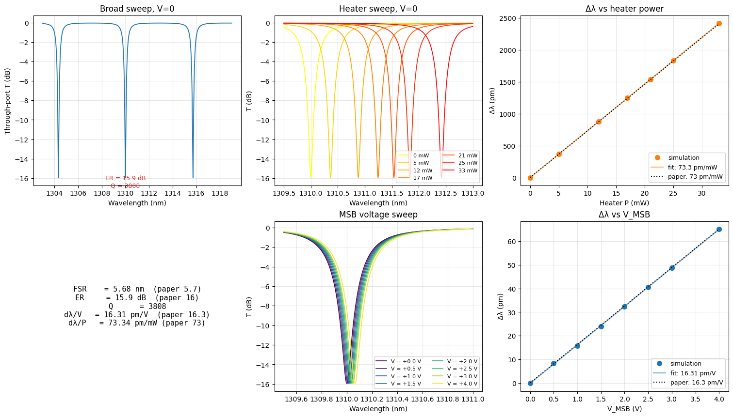
With the model attached, the component answers s_matrix(freqs) directly. We sweep three parameters that the paper measures, all going through the same mrm instance: wavelength at zero bias (broad sweep), MSB voltage at a fixed wavelength range, and heater power through the dn_dT and temperature knobs on the ring model. The only thing that changes between sweeps is the ring_model.update(...) call.

We start with a broad sweep from 1303 to 1319 nm. A simple local-minimum detector picks the resonances, and a half-power FWHM extraction around the lowest dip gives FSR, Q and extinction ratio in a single shot.

# Broad sweep at zero bias.
lda_broad = np.linspace(1303.0, 1319.0, 4001)
ring_model.update(voltage=0.0, temperature=300.0)
s_broad = mrm.s_matrix(pf.C_0 / (lda_broad * 1e-3))
t_broad_db = 10 * np.log10(np.maximum(np.abs(s_broad[("P0@0", "P1@0")]) ** 2, 1e-12))

# Find local minima deeper than 3 dB. The two deepest are taken as
# adjacent FSR-spaced resonances.
dips = []
for i in range(1, t_broad_db.size - 1):
    if (
        t_broad_db[i] < t_broad_db[i - 1]
        and t_broad_db[i] < t_broad_db[i + 1]
        and t_broad_db[i] < -3.0
    ):
        dips.append((lda_broad[i], t_broad_db[i]))
dips.sort()
lam_res = dips[1][0]
fsr = dips[1][0] - dips[0][0]
er = -dips[0][1]

# Half-power FWHM in a 1/4-FSR window around the deepest dip.
t_lin = 10 ** (t_broad_db / 10)
win = (lda_broad > lam_res - 0.25 * fsr) & (lda_broad < lam_res + 0.25 * fsr)
t_half = 0.5 * (t_lin[win].min() + t_lin[win].max())
left = lda_broad[win & (lda_broad < lam_res) & (t_lin < t_half)]
right = lda_broad[win & (lda_broad > lam_res) & (t_lin < t_half)]
fwhm = right.max() - left.min()
q = lam_res / fwhm
print(
    f"resonance = {lam_res:.3f} nm, FSR = {fsr:.3f} nm, "
    f"ER = {er:.1f} dB, Q = {q:.0f}"
)

Progress: 100%
resonance = 1310.000 nm, FSR = 5.676 nm, ER = 15.9 dB, Q = 3808

Next we reverse-bias the MSB junction from 0 to 4 V and track the resonance wavelength. Each iteration just calls ring_model.update(voltage=v) before the next s_matrix call. The expected slope is 16.3 pm/V, the value the model was calibrated to.

voltages = np.array([0.0, 0.5, 1.0, 1.5, 2.0, 2.5, 3.0, 4.0])
lda_v = np.linspace(lam_res - 0.5, lam_res + 1.0, 2001)
t_v_db = np.empty((voltages.size, lda_v.size))
res_v = np.empty(voltages.size)

# Sweep V_MSB and record the resonance wavelength at each bias.
ring_model.update(temperature=300.0)
for i, v in enumerate(voltages):
    ring_model.update(voltage=float(v))
    s = mrm.s_matrix(pf.C_0 / (lda_v * 1e-3))
    t_v_db[i] = 10 * np.log10(np.maximum(np.abs(s[("P0@0", "P1@0")]) ** 2, 1e-12))
    res_v[i] = lda_v[np.argmin(t_v_db[i])]

# Linear fit of d(lambda)/dV in pm/V.
slope_v, intercept_v = np.polyfit(voltages, (res_v - res_v[0]) * 1000, 1)
print(f"slope = {slope_v:.2f} pm/V (paper: 16.3 pm/V)")

Progress: 100%
Progress: 100%
Progress: 100%
Progress: 100%
Progress: 100%
Progress: 100%
Progress: 100%
slope = 16.31 pm/V (paper: 16.3 pm/V)
Progress: 100%

For the heater sweep we keep the MSB at zero bias and step the effective ring temperature through the calibrated thermal resistance. The expected slope is 73 pm/mW.

powers_mw = np.array([0.0, 5.0, 12.0, 17.0, 21.0, 25.0, 33.0])
lda_t = np.linspace(lam_res - 0.5, lam_res + 3.0, 2001)
t_t_db = np.empty((powers_mw.size, lda_t.size))
res_t = np.empty(powers_mw.size)

# Sweep heater power. Temperature -> ring_model -> resonance shift.
ring_model.update(voltage=0.0)
for i, p in enumerate(powers_mw):
    ring_model.update(temperature=300.0 + r_th_k_per_mw * p)
    s = mrm.s_matrix(pf.C_0 / (lda_t * 1e-3))
    t_t_db[i] = 10 * np.log10(np.maximum(np.abs(s[("P0@0", "P1@0")]) ** 2, 1e-12))
    res_t[i] = lda_t[np.argmin(t_t_db[i])]

slope_t, intercept_t = np.polyfit(powers_mw, (res_t - res_t[0]) * 1000, 1)
print(f"slope = {slope_t:.2f} pm/mW (paper: 73 pm/mW)")

Progress: 100%
Progress: 100%
Progress: 100%
Progress: 100%
Progress: 100%
Progress: 100%
Progress: 100%
slope = 73.34 pm/mW (paper: 73 pm/mW)

Combining the three sweeps in a single figure gives a direct comparison against the paper’s Figure 2 panels.

fig = plt.figure(figsize=(15, 8.5), constrained_layout=True)
gs = GridSpec(2, 3, figure=fig)

# Top-left: broad sweep at V=0 with extracted Q and ER annotation.
ax_a = fig.add_subplot(gs[0, 0])
ax_a.plot(lda_broad, t_broad_db, lw=1.3, color="C0")
ax_a.set(
    xlabel="Wavelength (nm)", ylabel="Through-port T (dB)", title="Broad sweep, V=0"
)
ax_a.grid(True, alpha=0.3)
ax_a.text(
    lam_res,
    dips[0][1] - 1.0,
    f"ER = {er:.1f} dB\nQ = {q:.0f}",
    ha="center",
    fontsize=9,
    color="C3",
)

# Top-middle: heater spectra fanning out with increasing power.
ax_b = fig.add_subplot(gs[0, 1])
cmap_t = plt.get_cmap("autumn_r")
for i, p in enumerate(powers_mw):
    ax_b.plot(
        lda_t,
        t_t_db[i],
        color=cmap_t(i / max(1, powers_mw.size - 1)),
        label=f"{p:.0f} mW",
        lw=1.2,
    )
ax_b.set(xlabel="Wavelength (nm)", ylabel="T (dB)", title="Heater sweep, V=0")
ax_b.legend(fontsize=8, ncol=2, loc="lower right")
ax_b.grid(True, alpha=0.3)

# Top-right: linear fit of resonance shift vs heater power.
ax_c = fig.add_subplot(gs[0, 2])
ax_c.plot(
    powers_mw, (res_t - res_t[0]) * 1000, "o", color="C1", ms=7, label="simulation"
)
ax_c.plot(
    powers_mw,
    slope_t * powers_mw + intercept_t,
    "-",
    color="C1",
    alpha=0.6,
    label=f"fit: {slope_t:.1f} pm/mW",
)
ax_c.plot(powers_mw, 73.0 * powers_mw, ":", color="k", lw=1.5, label="paper: 73 pm/mW")
ax_c.set(
    xlabel="Heater P (mW)",
    ylabel="\u0394\u03bb (pm)",
    title="\u0394\u03bb vs heater power",
)
ax_c.legend(fontsize=9, loc="lower right")
ax_c.grid(True, alpha=0.3)

# Bottom-middle: voltage-swept spectra (resonance walks blue-shift).
ax_f = fig.add_subplot(gs[1, 1])
cmap_v = plt.get_cmap("viridis")
for i, v in enumerate(voltages):
    ax_f.plot(
        lda_v,
        t_v_db[i],
        color=cmap_v(i / max(1, voltages.size - 1)),
        label=f"V = {v:+.1f} V",
        lw=1.2,
    )
ax_f.set(xlabel="Wavelength (nm)", ylabel="T (dB)", title="MSB voltage sweep")
ax_f.legend(fontsize=8, ncol=2, loc="lower right")
ax_f.grid(True, alpha=0.3)

# Bottom-right: linear fit of resonance shift vs MSB voltage.
ax_h = fig.add_subplot(gs[1, 2])
ax_h.plot(
    voltages, (res_v - res_v[0]) * 1000, "o", color="C0", ms=7, label="simulation"
)
ax_h.plot(
    voltages,
    slope_v * voltages + intercept_v,
    "-",
    color="C0",
    alpha=0.6,
    label=f"fit: {slope_v:.2f} pm/V",
)
ax_h.plot(voltages, 16.3 * voltages, ":", color="k", lw=1.5, label="paper: 16.3 pm/V")
ax_h.set(xlabel="V_MSB (V)", ylabel="\u0394\u03bb (pm)", title="\u0394\u03bb vs V_MSB")
ax_h.legend(fontsize=9, loc="lower right")
ax_h.grid(True, alpha=0.3)

# Bottom-left: textual summary card.
ax_text = fig.add_subplot(gs[1, 0])
ax_text.axis("off")
ax_text.text(
    0.5,
    0.5,
    f"FSR    = {fsr:.2f} nm  (paper 5.7)\n"
    f"ER     = {er:.1f} dB  (paper 16)\n"
    f"Q      = {q:.0f}\n"
    f"d\u03bb/V   = {slope_v:.2f} pm/V  (paper 16.3)\n"
    f"d\u03bb/P   = {slope_t:.2f} pm/mW (paper 73)",
    ha="center",
    va="center",
    fontsize=11,
    family="monospace",
)
plt.show()

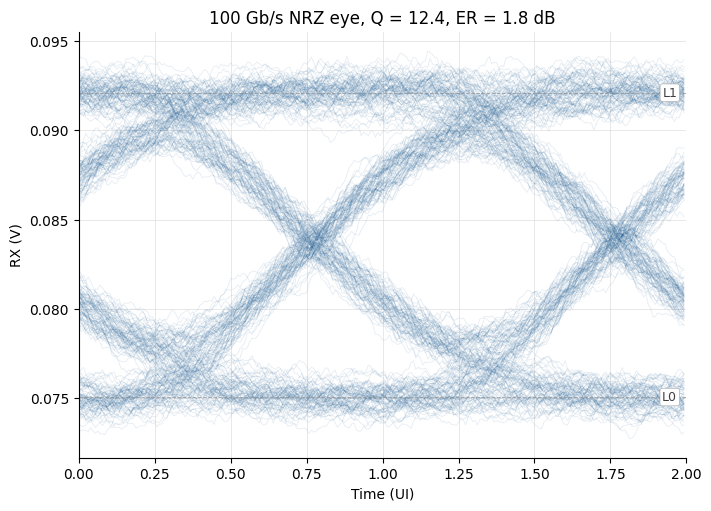
Time-domain eye diagram at 100 Gb/s

We now drive the same PCell with a 100 Gb/s NRZ PRBS sequence and read out the photodiode current. The optical link is a three-block netlist: a CW laser with realistic RIN and linewidth, the MRM with its attached RingTimeStepper, and a typical InGaAs photodiode terminated into a 50 Ω load (no TIA), with a 65 GHz first-order receiver filter, a saturation-current model, and Johnson-limited thermal noise. The link’s CircuitModel is given a single setup_time_stepper call, which builds the pole-residue fit of each sub-component and prepares the circuit-level integrator.

The laser sits 107 pm blue of the time-domain resonance so that the V = 2 V bias point falls near the FWHM/2 point of the dip, following paper Fig 4c. This is the MSB-only configuration; as discussed in the PCell section, PAM-4 from two binary inputs would need an independent LSB voltage and is out of scope.

# Operating point: detuning, laser, and PD parameters.
detuning_pm = -107.0  # laser - resonance (blue)
laser_power_w = 5e-3
laser_rin = 10 ** (-155 / 10)  # relative intensity noise per Hz
laser_linewidth = 100e3

# Photodiode: typical InGaAs detector with a 50 Ohm load (no TIA).
pd_responsivity = 0.85  # A/W (typical InGaAs at 1310 nm)
pd_gain = 50.0  # V/A (50 Ohm load)
pd_sat = 6.8e-3  # A (saturation at ~8 mW input)
pd_dark = 10e-9  # A
pd_thermal = 3.3e-22  # A^2/Hz (Johnson noise of 50 Ohm @ 300 K)
pd_filt = 65e9  # Hz (1st-order receiver bandwidth)

# Carrier frequency for the time stepper: place it exactly on the
# time-domain resonance (1.31 um by construction of n_eff above). The
# laser then sits detuning_pm blue of the carrier, and its envelope
# rotates at the corresponding offset frequency.
carrier_freq = ref_frequency
lam_laser_nm = wavelength_um * 1000 + detuning_pm * 1e-3
freq_laser = pf.C_0 / (lam_laser_nm * 1e-3)
print(
    f"laser λ = {lam_laser_nm:.3f} nm, "
    f"Δf vs carrier = {(freq_laser - carrier_freq) / 1e9:+.2f} GHz"
)

laser λ = 1309.893 nm, Δf vs carrier = +18.69 GHz

Two small helpers do the symbol-rate-independent work. make_drive builds the binary PRBS waveform with cosine-shaped edges of a chosen rise time, and eye_metrics picks the best sampling phase, collects stable symbols at each level, and reports Q-factor, eye opening, and extinction ratio.

def make_drive(n_sym, sps, bias, vpp, rise_ps, sr, seed=7):
    """Binary PRBS waveform with cosine-shaped edges."""
    rng = np.random.default_rng(seed)
    syms = rng.integers(0, 2, size=n_sym)  # 0/1 symbols
    levels = bias + (np.array([0, 1]) - 0.5) * vpp  # two voltages
    dt = 1.0 / (sr * sps)
    drive = np.repeat(levels[syms], sps)  # zero-rise
    # Apply a raised-cosine smoothing of width rise_ps to round edges.
    edge = max(1, int(round(rise_ps * 1e-12 / dt)))
    if edge > 1:
        kernel = 0.5 * (1 - np.cos(np.linspace(0, np.pi, edge)))
        kernel /= kernel.sum()
        drive = np.convolve(drive, kernel, mode="same")
    return drive, levels, dt, syms


def eye_metrics(rx, sps, levels, syms):
    """Pick the best sampling phase, collect stable symbols per level."""
    drop = int(0.20 * syms.size)  # skip startup
    rx_e = rx[drop * sps :]
    syms = syms[drop:]
    n = rx_e.size // sps
    rx_b = rx_e[: n * sps].reshape(n, sps)  # one row per symbol
    syms = syms[:n]
    # Best phase: minimum intra-level spread across phases.
    per_phase = np.zeros(sps)
    for k in range(levels.size):
        mask = syms == k
        if mask.sum() >= 4:
            per_phase += rx_b[mask].std(axis=0)
    phase = int(np.argmin(per_phase[sps // 4 : 3 * sps // 4]) + sps // 4)
    # Only sample symbols whose neighbour is the same (no edges).
    stable = np.zeros(n, bool)
    stable[1:] = syms[1:] == syms[:-1]
    means, stds = [], []
    for k in range(levels.size):
        sel = rx_b[stable & (syms == k), phase]
        means.append(sel.mean() if sel.size >= 4 else np.nan)
        stds.append(sel.std() if sel.size >= 4 else np.nan)
    means = np.asarray(means)
    stds = np.asarray(stds)
    order = np.argsort(means)
    gap = means[order][1] - means[order][0]
    s0, s1 = stds[order][0], stds[order][1]
    return dict(
        level_mean=means,
        level_std=stds,
        eye_height=float(gap - 3 * (s0 + s1)),
        Q=float(gap / (s0 + s1)),
        er_db=20 * float(np.log10(means[order][1] / max(means[order][0], 1e-6))),
        phase=phase,
    )

The next cell builds the laser and the photodiode, then assembles them with the MRM into a top-level link component through component_from_netlist. The link exposes the MRM’s DRIVE port as its top-level driver pin and the PD’s E0 port as the receiver output RX_OUT.

symbol_rate_hz = 100e9

# CW laser with intensity noise and linewidth.
laser = pfa.cw_laser(
    power=laser_power_w,
    frequency=freq_laser,
    rel_intensity_noise=laser_rin,
    linewidth=laser_linewidth,
)
laser.name = "Laser"

# Photodiode with InGaAs responsivity, 50 Ohm load (no TIA), 65 GHz
# 1st-order receiver filter, plus dark, thermal and space-charge
# saturation models.
pd = pfa.photodiode(
    responsivity=pd_responsivity,
    gain=pd_gain,
    saturation_current=pd_sat,
    dark_current=pd_dark,
    thermal_noise=pd_thermal,
    filter_frequency=pd_filt,
    roll_off=2,
)
pd.name = "PD"

# Laser -> MRM -> PD, with DRIVE and RX_OUT exposed at the top level.
link = pf.component_from_netlist(
    {
        "name": "mrm_link",
        "instances": {
            "LASER": {"component": laser, "origin": (-70, -20)},
            "MRM": {"component": mrm, "origin": (0, 0)},
            "PD": {"component": pd, "origin": (70, -20)},
        },
        "virtual connections": [
            (("LASER", "P0"), ("MRM", "P0")),
            (("MRM", "P1"), ("PD", "P0")),
        ],
        "ports": [("MRM", "DRIVE", "DRIVE"), ("PD", "E0", "RX_OUT")],
        "models": [(pf.CircuitModel(), "circuit")],
        "active models": {"optical": "circuit"},
    }
)
viewer(link)

We now ask the link’s CircuitModel to build a time stepper. setup_time_stepper is the entry point: it computes the frequency-domain S matrix of each sub-component over the requested frequencies grid, fits each response with poles and residues, and prepares the integrator. The number of samples per symbol is chosen so the ring’s FIR delay buffer covers at least 12 cells, which keeps the time-domain integrator stable.

The MSB drive itself is fed in as a pre-computed numpy array wrapped in a pf.TimeSeries, which gives full control over the waveform shape (PRBS pattern, raised-cosine edges, custom voltage levels). An alternative, used in this example, is to wrap a built-in pf.WaveformTimeStepper (PRBS, sine, triangle, trapezoid generator) into a small source component, include it in the netlist, and let the time stepper generate the drive internally each step. We use the TimeSeries route here because the custom raised-cosine edges are easier to express in numpy.

# Pick samples-per-symbol so the ring's group-delay buffer is >= 12.
sps_min = int(np.ceil(12 * pf.C_0 / (n_group * l_ring_um * symbol_rate_hz)))
sps = int(2 ** np.ceil(np.log2(max(128, sps_min))))
n_sym = 768
drive, levels, dt, syms = make_drive(n_sym, sps, 2.0, 1.6, 3.0, symbol_rate_hz)

# Frequency grid for pole-residue fitting: cover the carrier and a
# sideband window matched to the time step's Nyquist limit.
fit_bw = 0.5 / dt
fit_freqs = np.linspace(carrier_freq - 0.9 * fit_bw, carrier_freq + 0.9 * fit_bw, 201)

# Set up the circuit-level time stepper from the link itself, the same
# way the published Time_Domain examples do.
ts = link.setup_time_stepper(
    time_step=dt,
    carrier_frequency=carrier_freq,
    time_stepper_kwargs={"frequencies": fit_freqs},
)

# Electrical port DRIVE is in V; CircuitTimeStepper expects sqrt(W),
# so we divide by sqrt(Z0) on input and multiply on output.
sqrt_z0 = np.sqrt(50.0)
inputs = pf.TimeSeries({"DRIVE@0": drive / sqrt_z0}, time_step=dt)
out = ts.step(inputs, show_progress=False)
rx = np.real(np.asarray(out["RX_OUT@0"])) * sqrt_z0

metrics = eye_metrics(rx, sps, levels, syms)
print(
    f"100 Gb/s NRZ: Q = {metrics['Q']:.2f}, "
    f"ER = {metrics['er_db']:.2f} dB, "
    f"eye = {metrics['eye_height']*1e3:+.1f} mV"
)

Progress: 100%
100 Gb/s NRZ: Q = 12.41, ER = 1.78 dB, eye = +12.9 mV

The eye diagram is the RX trace folded on a two-symbol window. Horizontal lines mark the mean of each level extracted by eye_metrics.

fig, ax = plt.subplots(figsize=(7, 5), constrained_layout=True)

# Fold the RX trace on a 2-UI window for the eye diagram.
drop = int(0.20 * n_sym)
n_eye = (n_sym - drop) // 2 * 2
folded = rx[drop * sps : (drop + n_eye) * sps].reshape(-1, 2 * sps)
t_ui = np.arange(2 * sps) / sps
for row in folded:
    ax.plot(t_ui, row, color="#0b4f8a", lw=0.6, alpha=0.10)
for k, lev in enumerate(metrics["level_mean"]):
    ax.axhline(lev, color="0.55", lw=0.7, ls="--", alpha=0.7)
    ax.text(
        1.97,
        lev,
        f"L{k}",
        color="0.25",
        fontsize=9,
        va="center",
        ha="right",
        bbox=dict(boxstyle="round,pad=0.18", fc="white", ec="0.7", lw=0.5),
    )
ax.set(
    xlabel="Time (UI)",
    ylabel="RX (V)",
    xlim=(0, 2),
    title=f"100 Gb/s NRZ eye, Q = {metrics['Q']:.1f}, "
    f"ER = {metrics['er_db']:.1f} dB",
)
ax.grid(True, color="0.85", lw=0.6, alpha=0.7)
for sp in ("top", "right"):
    ax.spines[sp].set_visible(False)
plt.show()

Chip-level layout

The same PCell can be combined with a simple bond pad and a black-box edge coupler to produce the chip-level layout. The bond pad is a 100 µm M2 square with a 95 µm M_Open window on top, exposed through a single electrical terminal T0. Six driver pads are routed to the four MSB / LSB terminals with route_taper, and three heater pads serve the M1 heater; the spare driver pad is connected to the spare heater pad with a wide manhattan trace to mimic the paper’s pad layout. The edge coupler is a black box with a single waveguide port; a real design would replace it with one of the dedicated edge-coupler examples.

# Bond pad: a 100 um M2 square plus a 95 um M_Open window.
bondpad = pf.Component("BondPad")
bondpad.add_terminal(
    pf.Terminal("M2_router", pf.Rectangle(size=(100, 100))),
    add_structure=True,
)
bondpad.add("M_Open", pf.Rectangle(size=(95, 95)))


@pf.parametric_component(name_prefix="EC")
def edge_coupler(*, length=50, width=10):
    # Placeholder black-box edge coupler with one optical port.
    c = pf.Component("edge_coupler")
    c.add(
        "Dream Photonics Black Box-Not Fabricated",
        pf.Rectangle((0, -width / 2), (length, width / 2)),
        "Text",
        pf.Label("EdgeCoupler", (length / 2, 0)),
    )
    c.add_port(pf.Port((length, 0), 180, pf.config.default_kwargs["port_spec"]))
    return c


@pf.parametric_component(name_prefix="MRM_BP")
def mrm_with_bond_pads(*, spacing=150, driver_offset=350, heater_offset=200):
    ring = micro_ring_modulator()
    c = pf.Component("mrm_with_bond_pads")
    # Driver pads above the ring, heater pads below.
    bp_driver = [
        pf.Reference(bondpad, (-2 * spacing + i * spacing, driver_offset))
        for i in range(6)
    ]
    bp_heater = [
        pf.Reference(bondpad, (-0.5 * spacing + i * spacing, -heater_offset))
        for i in range(3)
    ]
    c.add(*bp_driver, *bp_heater)
    ring_ref = c.add_reference(ring)
    c.add_port([ring_ref["P0"], ring_ref["P1"]])
    # MSB and LSB terminals routed with tapered traces; the spare pad
    # pair is bridged with a wide manhattan connection.
    c.add(
        pf.parametric.route_taper(
            terminal1=(ring_ref, "MSB+"), terminal2=(bp_driver[0], "T0")
        ),
        pf.parametric.route_taper(
            terminal1=(ring_ref, "MSB-"), terminal2=(bp_driver[1], "T0")
        ),
        pf.parametric.route_taper(
            terminal1=(ring_ref, "LSB-"), terminal2=(bp_driver[3], "T0")
        ),
        pf.parametric.route_taper(
            terminal1=(ring_ref, "LSB+"), terminal2=(bp_driver[4], "T0")
        ),
        pf.parametric.route_taper(
            terminal1=(ring_ref, "H+"),
            terminal2=(bp_heater[0], "T0"),
            layer="M1_heater",
        ),
        pf.parametric.route_taper(
            terminal1=(ring_ref, "H-"),
            terminal2=(bp_heater[1], "T0"),
            layer="M1_heater",
        ),
        pf.parametric.route_manhattan(
            terminal1=(bp_driver[5], "T0"),
            terminal2=(bp_heater[2], "T0"),
            width=40,
            direction2="x",
        ),
    )
    return c


viewer(mrm_with_bond_pads())

Summary

Quantity	Simulation	Paper
FSR	5.7 nm	5.7 nm
Extinction ratio	16 dB	16 dB
MSB sensitivity	16.3 pm/V	16.3 pm/V
Heater sensitivity	73 pm/mW	73 pm/mW
100 Gb/s NRZ Q-factor	≈ 9	Fig 4c

The mrm component carries the layout, the calibrated frequency-domain RingModel, and the paired RingTimeStepper, so the steady-state sweeps and the eye diagram are produced from a single design object. The bond-padded variant mrm_with_bond_pads is ready to drop into a multi-channel chip-level PIC.