Inverse Design with Autograd

In the inverse design approach, instead of tuning a photonic geometry by hand, we specify a figure of merit and let a gradient-based optimizer discover the design parameters. The key ingredient is the adjoint method: the derivatives of the figure of merit with respect to all design parameters are obtained at the cost of a single extra simulation, no matter how many parameters there are.

Starting in version 1.4.4, PhotonForge integrates with Autograd to compute those derivatives automatically: the S matrix of a parametric component can be differentiated with respect to the component parameters through Tidy3D’s adjoint solver.

In this guide we apply inverse design in its simplest, parametric form: we create a differentiable 1×2 MMI splitter and use the automatic gradients to maximize its transmission with respect to the MMI dimensions. The same machinery scales unchanged to many-parameter freeform problems, as in the Inverse Design Grating Coupler example.

import autograd as ag
import autograd.numpy as np  # Important to import autograd's numpy module for tracing derivatives
import photonforge as pf
from matplotlib import pyplot as plt
import tidy3d as td

td.config.logging.level = "ERROR"
pf.config.default_technology = pf.basic_technology()

Differentiable Parametric Component

Components created with the parametric_component decorator support automatic differentiation out of the box: when the decorated function is called with parameters that are being traced by Autograd, it automatically returns a differentiable version of the component. The function body requires no changes whatsoever: it always receives plain numerical values, so we are free to use regular geometry operations and model setup inside, as usual.

Only two requirements apply:

• Differentiable parameters must be passed directly as scalars or arrays. Traced values nested inside lists, tuples, or dictionaries are not supported.

• The component must have an active Tidy3DModel, which is responsible for the gradient computation.

The splitter below is drawn with the stencil.mmi helper and has two design parameters: the length and the width of the MMI body. Note that the overall footprint of the component is kept fixed: the access waveguide length compensates changes in the MMI length, and the output separation is set explicitly instead of following the MMI width. Gradients are computed for the structures inside the simulation, so the ports (and the monitors derived from them), detected automatically at the fixed component edges, must not move when the parameters change.

total_length = 14.0
arm_sep = 1.5


@pf.parametric_component
def mmi_splitter(*, mmi_length=8.0, mmi_width=3.5):
    c = pf.Component("MMI1x2")
    spec = pf.config.default_technology.ports["Strip"]
    port_width, _ = spec.path_profile_for("WG_CORE")

    # Access waveguides stretch to compensate the MMI length, keeping the
    # total footprint (and the port positions) fixed
    c.add(
        "WG_CORE",
        *pf.stencil.mmi(
            length=mmi_length,
            width=mmi_width,
            num_ports=(1, 2),
            port_length=0.5 * (total_length - mmi_length),
            port_width=port_width,
            tapered_width=0.8,
            port_separation=arm_sep,
        ),
    )
    c.add("WG_CLAD", pf.envelope(c, offset=1.0, trim_x_min=True, trim_x_max=True))

    c.add_port(c.detect_ports([spec]))
    c.add_model(
        pf.Tidy3DModel(
            grid_spec=10,
            port_symmetries=[("P0", "P2", "P1")],
            verbose=False,
        )
    )
    return c


component = mmi_splitter()
component

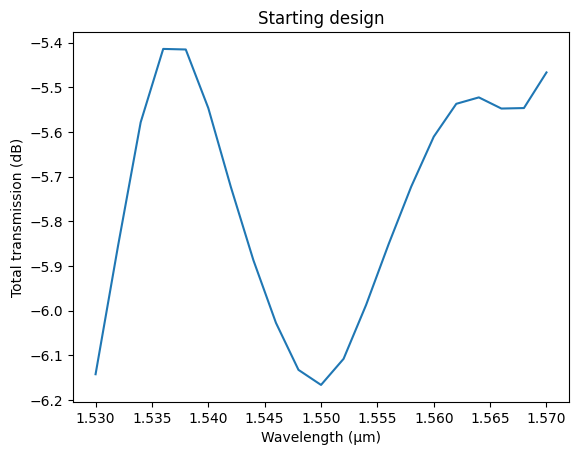
When called with plain values, the decorated function builds a regular component, so we can inspect the starting design as usual. We compute the baseline response over a 100 nm band, limiting the computation to the only input of interest through the inputs argument. The estimated cost gives an upper bound for each forward simulation (the adjoint simulation used in the gradient computation roughly doubles it).

wavelengths = np.linspace(1.53, 1.57, 21)
frequencies = pf.C_0 / wavelengths

model = component.select_active_model("optical")
print(f"Estimated cost: {model.estimate_cost(component, frequencies)}")

Estimated cost: 0.5511084862944671

s_baseline = component.s_matrix(frequencies, model_kwargs={"inputs": ["P0"]})

_, ax = plt.subplots(1, 1)
t_baseline = (
    np.abs(s_baseline[("P0@0", "P1@0")]) ** 2 + np.abs(s_baseline[("P0@0", "P2@0")]) ** 2
)
ax.plot(wavelengths, 10 * np.log10(t_baseline))
ax.set_xlabel("Wavelength (μm)")
ax.set_ylabel("Total transmission (dB)")
_ = ax.set_title("Starting design")

Differentiable S Matrix

To compute gradients, we need a scalar figure of merit. Optimizing at a single wavelength is usually not a good idea: it is easy to fall into narrowband resonant optima that perform well at the design wavelength and poorly everywhere else. Instead, we maximize the minimum transmission across the wavelength window, sampled at a few points; the broadband forward simulation computes all of them at no extra cost.

A hard minimum is not differentiable, so we use a smooth approximation based on the log-sum-exp function, with a temperature parameter tau that controls how closely it hugs the true minimum. We implement it elementwise so that it supports the per-frequency values of the differentiable S matrix (tidy3d.plugins.autograd.smooth_min does not support them yet).

Three details are worth noting:

• All mathematical operations on the S matrix elements must use functions from autograd.numpy.

• Limiting inputs to the excited port avoids paying for source excitations that do not contribute to the objective.

• The splitter is mirror-symmetric for every parameter value, so the two outputs are identical and the total transmitted power is simply twice the power in one arm. Using a single output in the objective also reduces the gradient cost: the adjoint sources are grouped per port, so fewer ports in the objective means fewer adjoint simulations.

from tidy3d.config import config

# The volumetric field data used by the gradient computation grows with the number
# of wavelengths; reduce its in-plane sampling density to keep downloads fast
config.adjoint.monitor_interval_poly = (2, 2, 1)

freqs_opt = pf.C_0 / np.linspace(wavelengths[0], wavelengths[-1], 3)


def smooth_min(values, tau=0.02):
    """Differentiable approximation of min(values)."""
    return -tau * np.log(sum(np.exp(-v / tau) for v in values))


def worst_transmission(params):
    c = mmi_splitter(mmi_length=params[0], mmi_width=params[1])
    s = c.s_matrix(freqs_opt, show_progress=False, model_kwargs={"inputs": ["P0"]})
    t = 2 * np.abs(s[("P0@0", "P1@0")]) ** 2  # symmetric splitter: P2 mirrors P1
    return smooth_min(t)

The function value_and_grad from Autograd evaluates the objective and its gradient simultaneously. Behind the scenes, PhotonForge runs one forward and two adjoint FDTD simulations (one broadband adjoint per port involved in the objective), regardless of the number of parameters or wavelengths being differentiated.

params0 = np.array([8.0, 3.5])

value, gradient = ag.value_and_grad(worst_transmission)(params0)
print(f"min T = {value:.3f}, dT/d(length) = {gradient[0]:+.3f}, dT/d(width) = {gradient[1]:+.3f}")

min T = 0.258, dT/d(length) = +0.108, dT/d(width) = -1.180

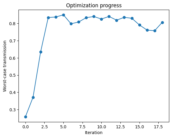
Gradient-Based Optimization

With gradients available, any gradient-based algorithm can drive the design. Here a few iterations of the Adam algorithm are enough for our 2-parameter splitter; for larger problems, dedicated optimizer packages such as Optax can be used in exactly the same way (see the Inverse Design Grating Coupler example).

The parameters are clipped after each update to keep the geometry valid; the same mechanism can be used to enforce fabrication constraints, such as minimal feature sizes. Note that simulation results are cached, so re-evaluating the objective at parameters that have already been simulated (like the initial ones above) adds no cost. Because the objective tracks the worst wavelength in the band, the trace can be slightly less regular than a single-frequency optimization (the active band edge may hop between iterations), and the converged response is flatter, at a slightly lower peak. With the coarse grid used in this demonstration, the objective fluctuates by a few percent near the optimum (re-meshing noise from sub-grid geometry changes), so the optimization trace plateaus with some scatter once converged. A finer grid (higher grid_spec) reduces this noise in production optimizations.

bounds = (np.array([4.0, 2.2]), np.array([12.0, 4.0]))
learning_rate = 0.1

value_and_grad = ag.value_and_grad(worst_transmission)
params = np.array(params0)
m = np.zeros_like(params)
v = np.zeros_like(params)
history = []

for i in range(1, 20):
    value, gradient = value_and_grad(params)
    history.append((params, value))
    print(f"Iteration {i:2}: min T = {value:.3f} at ({params[0]:.3f}, {params[1]:.3f})")
    # Adam update (gradient ascent)
    m = 0.9 * m + 0.1 * gradient
    v = 0.999 * v + 0.001 * gradient**2
    step = (m / (1 - 0.9**i)) / (np.sqrt(v / (1 - 0.999**i)) + 1e-8)
    params = np.clip(params + learning_rate * step, *bounds)

best_params, best_value = max(history, key=lambda h: h[1])
print(f"Best: min T = {best_value:.3f} at ({best_params[0]:.3f}, {best_params[1]:.3f})")

Iteration  1: min T = 0.258 at (8.000, 3.500)
Iteration  2: min T = 0.371 at (8.100, 3.400)
Iteration  3: min T = 0.635 at (8.194, 3.300)
Iteration  4: min T = 0.835 at (8.254, 3.208)
Iteration  5: min T = 0.838 at (8.317, 3.148)
Iteration  6: min T = 0.850 at (8.386, 3.099)
Iteration  7: min T = 0.798 at (8.458, 3.071)
Iteration  8: min T = 0.809 at (8.526, 3.076)
Iteration  9: min T = 0.834 at (8.593, 3.102)
Iteration 10: min T = 0.840 at (8.658, 3.137)
Iteration 11: min T = 0.826 at (8.717, 3.171)
Iteration 12: min T = 0.841 at (8.785, 3.207)
Iteration 13: min T = 0.819 at (8.832, 3.208)
Iteration 14: min T = 0.836 at (8.880, 3.192)
Iteration 15: min T = 0.830 at (8.928, 3.168)
Iteration 16: min T = 0.791 at (8.972, 3.149)
Iteration 17: min T = 0.762 at (9.011, 3.142)
Iteration 18: min T = 0.758 at (9.043, 3.147)
Iteration 19: min T = 0.806 at (9.074, 3.167)
Best: min T = 0.850 at (8.386, 3.099)

_, ax = plt.subplots(1, 1)
ax.plot([h[1] for h in history], "o-")
ax.set_xlabel("Iteration")
ax.set_ylabel("Worst-case transmission")
_ = ax.set_title("Optimization progress")

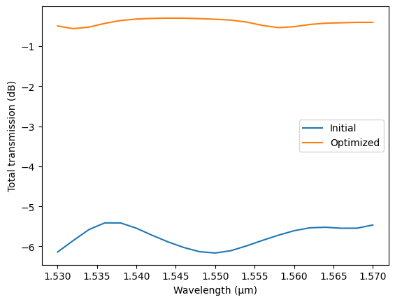
Finally, we compare the optimized splitter to the starting design over the full band. The optimized component is created with plain values, so this is a regular S matrix computation.

optimized = mmi_splitter(mmi_length=float(best_params[0]), mmi_width=float(best_params[1]))
s_optimized = optimized.s_matrix(frequencies, model_kwargs={"inputs": ["P0"]})

t_optimized = (
    np.abs(s_optimized[("P0@0", "P1@0")]) ** 2 + np.abs(s_optimized[("P0@0", "P2@0")]) ** 2
)

_, ax = plt.subplots(1, 1)
ax.plot(wavelengths, 10 * np.log10(t_baseline), label="Initial")
ax.plot(wavelengths, 10 * np.log10(t_optimized), label="Optimized")
ax.set_xlabel("Wavelength (μm)")
ax.set_ylabel("Total transmission (dB)")
_ = ax.legend()

optimized

Fine-Tuning the Gradient Computation

PhotonForge maps perturbations of the user parameters to changes in the simulation geometry through local finite differences. These are computed directly on the geometry, without any extra electromagnetic simulations, but the step sizes can matter when a parameter has a very small or very large scale. They can be controlled, globally or per parameter, through the model’s autograd configuration:

from photonforge.models.tidy3d import Tidy3DAutogradConfig

model = pf.Tidy3DModel(
    autograd_config=Tidy3DAutogradConfig(
        relative_diff_step={"mmi_length": 1e-3},
        absolute_diff_step=1e-6,
    )
)

The configuration also exposes exclude_domain_spanning_structures (enabled by default), which excludes structures that span the simulation domain, such as substrate and cladding layers, from the gradient computation.

A few limitations apply to the current implementation:

• Gradients are computed with the geometric method only, which differentiates the boxes and polygons that the parameters affect. A permittivity-based method is planned for a future release.

• Only the Tidy3DModel supports differentiable S matrices for now.

• As mentioned before, traced parameters must be scalars or arrays passed directly to the parametric function, and port positions should not depend on them.

Gradient-based optimization is local by nature, so it pairs well with statistical exploration: a Monte Carlo sweep of the design space (see the random variables support in parametric_technology and the pf.monte_carlo module) can locate promising starting points, from which a few Autograd iterations efficiently converge to the local optimum.

See also:

• Custom Parametric Components

• S Parameters

• Tidy3D Model

• Inverse Design Grating Coupler