Electrical Filter

Between the pattern generator and the modulator, and between the photodiode and the decision circuit, electrical signals are shaped by filters: drivers and amplifiers band-limit them, matching networks and packages add their own responses, and equalizers deliberately reshape them. The FilterTimeStepper brings this signal conditioning into time-domain simulations as a two-port electrical block that filters whatever passes through it.

The family argument selects the response type, and the table below summarizes the options:

family	Type	Key arguments	Typical use
"rc"	Analog, first order	f_cutoff	Simple RC pole: pad, junction, or driver roll-off
"butterworth"	Analog	f_cutoff, order	Maximally flat passband
"bessel"	Analog	f_cutoff, order	Nearly linear phase: pulses without ringing
"cheby1"	Analog	f_cutoff, order, ripple	Sharpest roll-off, at the cost of passband ripple
"rectangular"	FIR, windowed sinc	f_cutoff, taps, window	Brick-wall approximations
"gaussian"	FIR	f_cutoff, taps	Gaussian pulse shaping without overshoot
"digital"	FIR or IIR	b, a	Arbitrary user-designed responses

The frequency-selective families also take a shape of low-pass ("lp"), high-pass ("hp"), band-pass ("bp"), or band-stop ("bs"), and insertion_loss adds a flat attenuation to any of them. This guide measures the filter responses with a single impulse per filter, compares the classic families in the frequency and time domains, and shows how to bring a custom digital design into the simulation.

Setup

import matplotlib.pyplot as plt
import numpy as np
from scipy import signal
import photonforge as pf
import photonforge.abstract as pfa

viewer = pf.live_viewer.LiveViewer()

LiveViewer started at http://localhost:52776

tech = pf.basic_technology()
pf.config.default_technology = tech

f0 = pf.C_0 / 1.55
z0 = 50.0
time_step = 0.5e-12
num_steps = 4096

Measuring a Filter Response

The abstract filter component has an input port E0 and an output port E1 (filtering runs from the first port to the second, in sorted order). Since the filter is linear, its entire frequency response can be measured with one simulation: run the time stepper directly on the component, inject a single-sample unit impulse through a TimeSeries keyed by its input port, and Fourier-transform the output. We wrap this measurement in a small helper because every section of the guide uses it.

example_filter = pfa.filter(family="butterworth", f_cutoff=20e9, order=4)
viewer(example_filter)

freqs = np.fft.rfftfreq(num_steps, time_step)


def frequency_response(filter_component):
    # Inject a unit impulse directly into the filter and Fourier-transform the output
    v_in = np.zeros(num_steps)
    v_in[0] = 1.0
    time_stepper = filter_component.setup_time_stepper(
        time_step=time_step, carrier_frequency=f0, show_progress=False
    )
    output = time_stepper.step(inputs=pf.TimeSeries({"E0@0": v_in}, time_step), show_progress=False)
    return np.fft.rfft(np.real(output["E1@0"]))

The Classic Analog Families

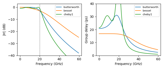
Filter design is always a compromise between how sharply the response falls and how cleanly signals pass through, and the classic families sit at different points of that trade-off. A fourth-order low-pass at 20 GHz from each family makes the comparison concrete: the Chebyshev response rolls off fastest at the price of passband ripple, the Butterworth response is maximally flat, and the Bessel response gives up steepness for a nearly linear phase. The right panel shows the group delay, \(-\mathrm{d} \angle H / \mathrm{d} \omega\), where the Bessel filter’s flat delay stands out: all frequency components of a pulse arrive together.

families = {
    "butterworth": {},
    "bessel": {},
    "cheby1": {"ripple": 1},
}

f_cutoff = 20e9
fig, (ax1, ax2) = plt.subplots(1, 2, figsize=(7, 3), tight_layout=True)
band = freqs < 60e9
for family, kwargs in families.items():
    h = frequency_response(pfa.filter(family=family, f_cutoff=f_cutoff, order=4, **kwargs))
    # Group delay from the unwrapped phase derivative
    delay = -np.gradient(np.unwrap(np.angle(h)), 2 * np.pi * freqs)
    ax1.plot(freqs[band] / 1e9, 20 * np.log10(np.abs(h[band])), label=family)
    ax2.plot(freqs[band] / 1e9, delay[band] * 1e12, label=family)

ax1.axvline(f_cutoff / 1e9, color="k", linestyle=":", linewidth=1)
ax1.set(xlabel="Frequency (GHz)", ylabel="$|H|$ (dB)", ylim=(-40, 3))
ax2.set(xlabel="Frequency (GHz)", ylabel="Group delay (ps)", ylim=(0, 40))
ax1.legend(fontsize=8)
_ = ax2.legend(fontsize=8)

Low-Pass, High-Pass, Band-Pass, and Band-Stop

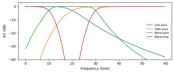
The shape argument transforms the same prototype into the four standard responses. Band-pass and band-stop shapes take a two-value f_cutoff sequence with the low and high band edges.

shapes = {
    "Low-pass": ("lp", 20e9),
    "High-pass": ("hp", 20e9),
    "Band-pass": ("bp", (10e9, 30e9)),
    "Band-stop": ("bs", (10e9, 30e9)),
}

fig, ax = plt.subplots(figsize=(7, 3), tight_layout=True)
for label, (shape, f_cutoff_shape) in shapes.items():
    h = frequency_response(
        pfa.filter(family="butterworth", shape=shape, f_cutoff=f_cutoff_shape, order=4)
    )
    ax.plot(freqs[band] / 1e9, 20 * np.log10(np.maximum(np.abs(h[band]), 1e-6)), label=label)

ax.set(xlabel="Frequency (GHz)", ylabel="$|H|$ (dB)", ylim=(-40, 3))
_ = ax.legend(fontsize=8)

Ringing vs Clean Settling in the Time Domain

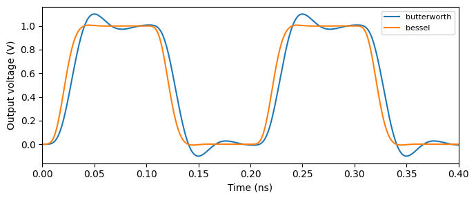
The group delay panel above has direct consequences for signals. Passing the same trapezoidal pulse train from a signal_source through the Butterworth and Bessel filters shows why receivers and drivers are usually specified with Bessel-like responses: the Butterworth filter’s sharper cutoff comes with overshoot and ringing on every edge, while the Bessel filter settles cleanly, only rounding the corners.

source = pfa.signal_source(
    frequency=5e9, amplitude=1 / np.sqrt(z0), waveform="trapezoid", width=0.5, rise=0.05, fall=0.05
)

fig, ax = plt.subplots(figsize=(7, 3), tight_layout=True)
pulse_steps = 800
t = np.arange(pulse_steps) * time_step
for i, family in enumerate(["butterworth", "bessel"]):
    # Source -> filter, with the filter output exposed
    link = pf.Component(f"pulse_link_{i}")
    source_ref = link.add_reference(source)
    filter_ref = link.add_reference(pfa.filter(family=family, f_cutoff=20e9, order=4))
    filter_ref.connect("E0", source_ref["E0"])
    link.add_port(filter_ref["E1"], "out")
    link.add_model(pf.CircuitModel(), "Circuit")

    time_stepper = link.setup_time_stepper(
        time_step=time_step, carrier_frequency=f0, show_progress=False
    )
    output = time_stepper.step(steps=pulse_steps, time_step=time_step, show_progress=False)
    ax.plot(t * 1e9, np.real(output["out@0"]) * np.sqrt(z0), label=family)

ax.set(xlabel="Time (ns)", ylabel="Output voltage (V)", xlim=(0, 0.4))
_ = ax.legend(fontsize=8)

Custom Digital Filters

The "digital" family accepts direct (b) and recursive (a) coefficients, so any response designed with standard tools can be dropped into the simulation: equalizers, channel models fitted to measurements, or FIR taps. One important detail: digital coefficients are applied once per simulation step, so they must be designed for a sampling rate of exactly \(1 / \Delta t\).

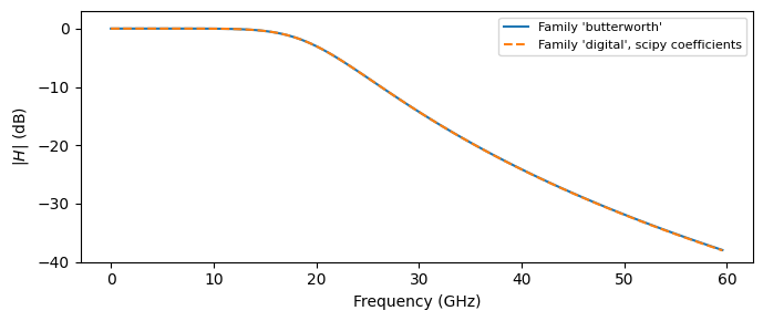
As a check, we design the same fourth-order 20 GHz Butterworth low-pass digitally with scipy.signal.butter at the simulation rate and compare it with the built-in analog family: the two responses lie on top of each other.

# Digital design at the simulation sampling rate
b_digital, a_digital = signal.butter(4, 20e9, btype="low", fs=1 / time_step)
h_digital = frequency_response(
    pfa.filter(family="digital", b=tuple(b_digital), a=tuple(a_digital))
)
h_analog = frequency_response(pfa.filter(family="butterworth", f_cutoff=20e9, order=4))

fig, ax = plt.subplots(figsize=(7, 3), tight_layout=True)
ax.plot(freqs[band] / 1e9, 20 * np.log10(np.abs(h_analog[band])), label="Family 'butterworth'")
ax.plot(
    freqs[band] / 1e9,
    20 * np.log10(np.abs(h_digital[band])),
    "--",
    label="Family 'digital', scipy coefficients",
)
ax.set(xlabel="Frequency (GHz)", ylabel="$|H|$ (dB)", ylim=(-40, 3))
_ = ax.legend(fontsize=8)

Summary

• pfa.filter is a two-port electrical filter: input on E0, output on E1; insertion_loss adds a flat attenuation on top of the response.

• The family argument covers the classic analog prototypes ("rc", "butterworth", "bessel", "cheby1" with order and ripple), windowed FIR types ("rectangular" with window and taps, "gaussian" for pulse shaping), and "digital" for arbitrary coefficients.

• shape selects low-pass, high-pass, band-pass, or band-stop; the band shapes take a two-value f_cutoff.

• Family choice is a trade-off between roll-off steepness and time-domain behavior: Chebyshev is sharpest with ripple, Butterworth is maximally flat, and Bessel’s linear phase (flat group delay) passes pulses without ringing.

• Digital coefficients run once per simulation step: design them for a sampling rate of \(1 / \Delta t\).

• A single injected impulse and an FFT measure the whole response of any linear block, a technique that works for any time stepper, not just filters.