Analytic MZI Model

The AnalyticMZIModel provides a compact, physically meaningful description of a 4-port Mach-Zehnder interferometer. It captures:

Feature	Parameters
Coupler splitting	\(\kappa_1\), \(\kappa_2\) (coupling), \(\tau_1\), \(\tau_2\) (transmission)
Propagation	\(n_\text{eff}\), \(n_\text{group}\) (per arm)
Arm lengths	\(\ell_1\), \(\ell_2\)
Dispersion	\(D\), \(S\) (per arm)
Loss	\(L_p\) (propagation loss), \(L_0\) (extra loss) per arm
Temperature sensitivity	\(\mathrm{d}n/\mathrm{d}T\), \(\mathrm{d}L_p/\mathrm{d}T\) per arm
Electro-optic modulation	\(V_{\pi L}\), \(\mathrm{d}L/\mathrm{d}V\), \(\mathrm{d}^2L/\mathrm{d}V^2\) per arm

The S matrix for each mode is:

\[S_{31} = \tau_1\, t_1\, \tau_2 + \kappa_1\, t_2\, \kappa_2\]

\[S_{41} = \tau_1\, t_1\, \kappa_2 + \kappa_1\, t_2\, \tau_2\]

\[S_{32} = \kappa_1\, t_1\, \tau_2 + \tau_1\, t_2\, \kappa_2\]

\[S_{42} = \kappa_1\, t_1\, \kappa_2 + \tau_1\, t_2\, \tau_2\]

where \(t_1\) and \(t_2\) are the arm transmissions computed from an AnalyticWaveguideModel-style formula, and \(\kappa\), \(\tau\) are the coupler coefficients. When tau is not specified, it is calculated from kappa as \(\tau = j\,e^{j\,\angle\kappa}\sqrt{1 - |\kappa|^2}\), ensuring a lossless unitary coupler.

This notebook walks through the model parameter by parameter, building intuition with black_box_component.

Setup

import matplotlib.pyplot as plt
import numpy as np
import photonforge as pf
import tidy3d as td

tech = pf.basic_technology()
pf.config.default_technology = tech

wavelengths = np.linspace(1.5, 1.6, 1001)
freqs = pf.C_0 / wavelengths
f0 = pf.C_0 / 1.55

Balanced MZI: Basic Operation

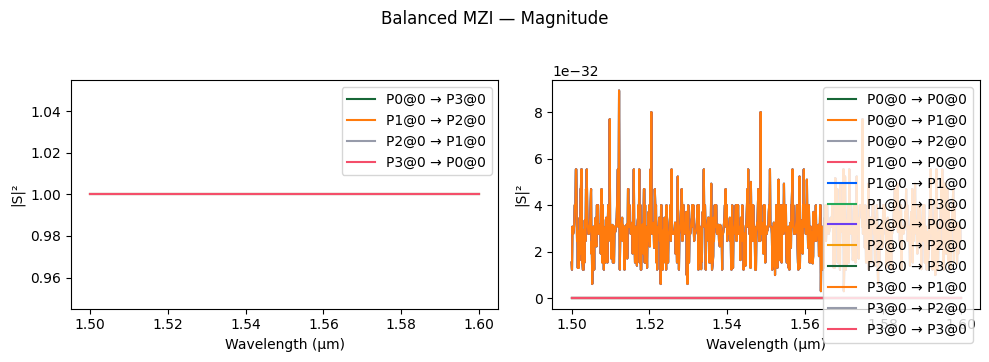
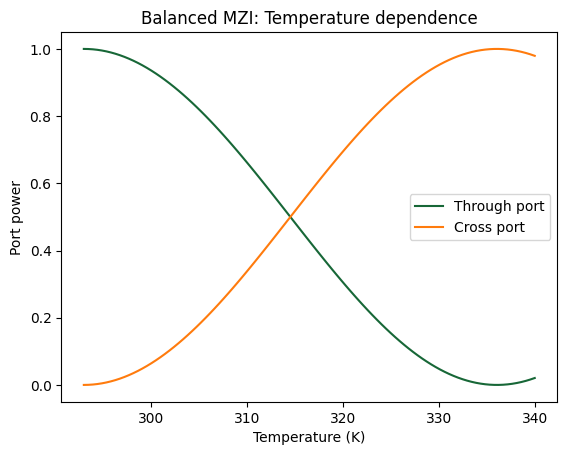
The simplest MZI has two arms of equal length and two identical 3 dB couplers (\(|\kappa|^2 = 0.5\)). When both arms are identical, the interference pattern is constant across wavelength. To demonstrate this non-trivially, we apply a temperature dependence to one arm and sweep the temperature, showing constant output power.

With balanced arms (\(\ell_1 = \ell_2\), identical \(n_\text{eff}\)), all the light exits from the cross port (port 3) and none from the through port (port 2).

model_balanced = pf.AnalyticMZIModel(
    n_eff1=2.4,
    n_eff2=2.4,
    n_group1=4.2,
    n_group2=4.2,
    length1=100,
    length2=100,
    dn1_dT=1.8e-4,
    reference_temperature=293.0,
    reference_frequency=f0,
)

bb_balanced = model_balanced.black_box_component(port_spec="Strip")
bb_balanced

s_balanced = bb_balanced.s_matrix(freqs, show_progress=False)

pf.plot_s_matrix(s_balanced)
plt.suptitle("Balanced MZI — Magnitude", y=1.02)
plt.show()

Note on parameter updates: In real-world photonic devices, only certain parameters can be dynamically updated after fabrication (e.g., temperature via heaters or voltage via electrodes). Other parameters like waveguide length, coupling coefficients, and material properties are fixed during manufacturing. Therefore, we use model_kwargs for dynamic parameters (temperature and voltage) but define new models in for loops for static parameters that cannot be changed post-fabrication.

temperatures = np.linspace(293, 340, 101)

through_powers = []
cross_powers = []

for T in temperatures:
    s = bb_balanced.s_matrix(
        [f0], model_kwargs={"temperature1": T}, show_progress=False
    )
    pn = sorted(s.ports)
    through_key = (f"{pn[0]}@0", f"{pn[3]}@0")
    cross_key = (f"{pn[0]}@0", f"{pn[2]}@0")
    through_powers.append(np.abs(s[through_key][0]) ** 2)
    cross_powers.append(np.abs(s[cross_key][0]) ** 2)

through_powers = np.array(through_powers)
cross_powers = np.array(cross_powers)

plt.figure()
plt.plot(temperatures, through_powers, label="Through port")
plt.plot(temperatures, cross_powers, label="Cross port")
plt.xlabel("Temperature (K)")
plt.ylabel("Port power")
plt.title("Balanced MZI: Temperature dependence")
plt.legend()
plt.show()

Arm Length Imbalance (\(\Delta L\))

The key design parameter of an MZI is the arm length difference \(\Delta L = \ell_2 - \ell_1\). This introduces a frequency-dependent phase difference between the two arms:

\[\Delta\phi = \frac{2\pi\, n_\text{group}\, \Delta L}{c_0}\,(f - f_0) + \frac{2\pi f_0}{c_0}n_\text{eff} \Delta L\]

Note the \(n_\text{group}\) dependence; the \(n_\text{eff}\) term is a constant (frequency-independent) phase. The free spectral range (FSR) — the spacing between successive peaks — is:

\[\text{FSR} \approx \frac{c_0}{n_\text{group}\, \Delta L}\]

Note that FSR is only a function of group index.

Below we compare MZIs with different arm length imbalances.

fig, axes = plt.subplots(1, 2, figsize=(12, 4))

delta_Ls = [0, 10, 20]
base_length = 100

base_model = pf.AnalyticMZIModel(
    n_eff1=2.4,
    n_eff2=2.4,
    n_group1=4.2,
    n_group2=4.2,
    length1=base_length,
    length2=base_length,
    reference_frequency=f0,
)

bb = base_model.black_box_component(port_spec="Strip")

for dL in delta_Ls:
    model = pf.AnalyticMZIModel(
        n_eff1=2.4,
        n_eff2=2.4,
        n_group1=4.2,
        n_group2=4.2,
        length1=base_length,
        length2=base_length + dL,
        reference_frequency=f0,
    )
    bb = model.black_box_component(port_spec="Strip")
    s = bb.s_matrix(freqs, show_progress=False)
    pn = sorted(s.ports)
    through_key = (f"{pn[0]}@0", f"{pn[3]}@0")
    cross_key = (f"{pn[0]}@0", f"{pn[2]}@0")

    label = f"$\\Delta L = {dL}$ µm"
    axes[0].plot(wavelengths, np.abs(s[through_key]) ** 2, label=label)
    axes[1].plot(wavelengths, np.abs(s[cross_key]) ** 2, label=label)

axes[0].set_xlabel("Wavelength (µm)")
axes[0].set_ylabel("$|S_{30}|^2$ (through)")
axes[0].set_title("Through port")
axes[0].legend()

axes[1].set_xlabel("Wavelength (µm)")
axes[1].set_ylabel("$|S_{20}|^2$ (cross)")
axes[1].set_title("Cross port")
axes[1].legend()

fig.tight_layout()
plt.show()

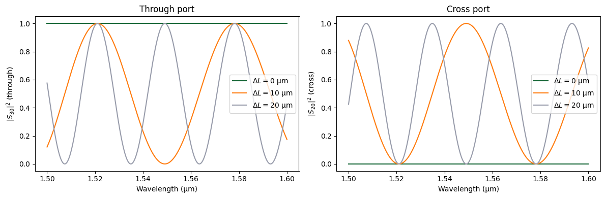
For non-zero \(\Delta L\), as \(\Delta L\) increases, the fringe period (FSR) decreases. A balanced MZI (\(\Delta L = 0\)) shows no fringes and the output is constant across wavelength.

Coupler Splitting Ratio

The default coupler is a 3 dB splitter (\(|\kappa|^2 = 0.5\)). Changing the coupling coefficient modifies the extinction ratio (ER) of the interference fringes.

Maximum extinction ratio is achieved when both couplers are exactly 3 dB. Any deviation reduces the fringe depth. Below we compare different coupling values.

fig, axes = plt.subplots(1, 2, figsize=(12, 4))

kappas = [-1j * k for k in [0.4, 0.5**0.5, 0.6, 0.9]]
kappa_labels = [
    "$|\\kappa|^2 = 0.16$",
    "$|\\kappa|^2 = 0.50$",
    "$|\\kappa|^2 = 0.36$",
    "$|\\kappa|^2 = 0.81$",
]

base_model = pf.AnalyticMZIModel(
    n_eff1=2.4,
    n_eff2=2.4,
    n_group1=4.2,
    n_group2=4.2,
    length1=100,
    length2=130,
    kappa1=-1j * 0.5**0.5,
    kappa2=-1j * 0.5**0.5,
    reference_frequency=f0,
)

bb = base_model.black_box_component(port_spec="Strip")

for kappa, label in zip(kappas, kappa_labels):
    model = pf.AnalyticMZIModel(
        n_eff1=2.4,
        n_eff2=2.4,
        n_group1=4.2,
        n_group2=4.2,
        length1=100,
        length2=130,
        kappa1=kappa,
        kappa2=kappa,
        reference_frequency=f0,
    )
    bb = model.black_box_component(port_spec="Strip")
    s = bb.s_matrix(freqs, show_progress=False)
    pn = sorted(s.ports)
    through_key = (f"{pn[0]}@0", f"{pn[3]}@0")
    cross_key = (f"{pn[0]}@0", f"{pn[2]}@0")

    axes[0].plot(
        wavelengths, 10 * np.log10(np.abs(s[through_key]) ** 2 + 1e-30), label=label
    )
    axes[1].plot(
        wavelengths, 10 * np.log10(np.abs(s[cross_key]) ** 2 + 1e-30), label=label
    )

for ax in axes:
    ax.set_xlabel("Wavelength (µm)")
    ax.set_ylim(-50, 1)

axes[0].set_ylabel("$|S_{31}|^2$ (dB)")
axes[0].set_title("Through port")
axes[0].legend(fontsize=8)

axes[1].set_ylabel("$|S_{41}|^2$ (dB)")
axes[1].set_title("Cross port")
axes[1].legend(fontsize=8)

fig.tight_layout()
plt.show()

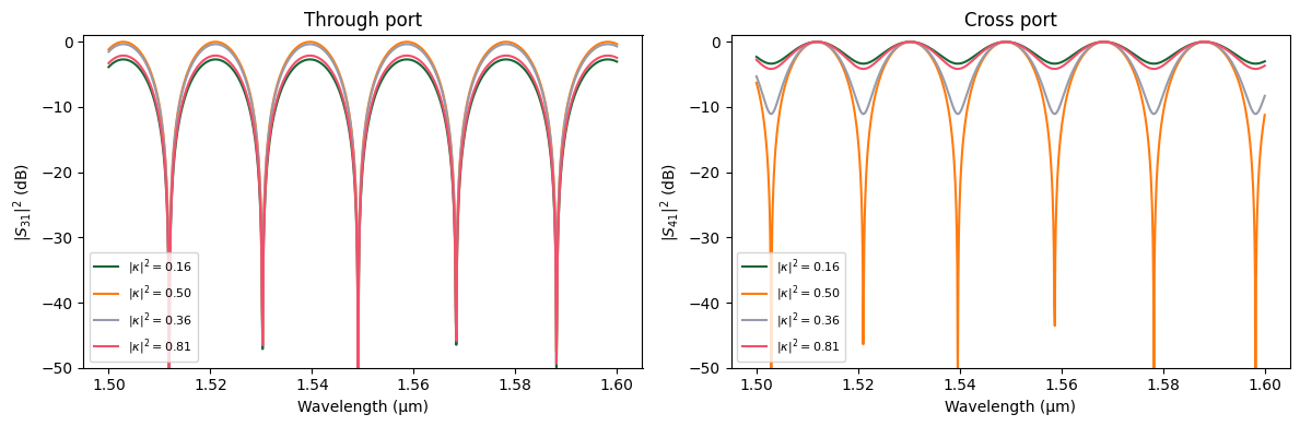
Only the 50:50 coupler (\(|\kappa|^2 = 0.5\)) achieves perfect extinction. Asymmetric splitting results in a shallower null because the two interfering fields no longer have equal magnitude.

Chromatic Dispersion

Like the AnalyticWaveguideModel, each arm of the MZI can include chromatic dispersion \(D\) and dispersion slope \(S\). Dispersion does not affect the peak-to-null contrast, but it curves the spectral response, making the FSR non-uniform across the band.

Below we compare a dispersion-free MZI with two dispersive cases.

fig, axes = plt.subplots(1, 2, figsize=(12, 4))

dispersions = [0, 2e-14, 4e-14]
labels = ["$D = 0$", "$D = 2 \\times 10^{-14}$", "$D = 4 \\times 10^{-14}$"]

base_model = pf.AnalyticMZIModel(
    n_eff1=2.4,
    n_eff2=2.4,
    n_group1=4.2,
    n_group2=4.2,
    length1=200,
    length2=250,
    dispersion1=0,
    dispersion2=0,
    reference_frequency=f0,
)

bb = base_model.black_box_component(port_spec="Strip")

for D, label in zip(dispersions, labels):
    model = pf.AnalyticMZIModel(
        n_eff1=2.4,
        n_eff2=2.4,
        n_group1=4.2,
        n_group2=4.2,
        length1=200,
        length2=250,
        dispersion1=D,
        dispersion2=D,
        reference_frequency=f0,
    )
    bb = model.black_box_component(port_spec="Strip")
    s = bb.s_matrix(freqs, show_progress=False)
    pn = sorted(s.ports)
    through_key = (f"{pn[0]}@0", f"{pn[3]}@0")
    cross_key = (f"{pn[0]}@0", f"{pn[2]}@0")

    axes[0].plot(wavelengths, np.abs(s[through_key]) ** 2, label=label)
    axes[1].plot(wavelengths, np.abs(s[cross_key]) ** 2, label=label)

axes[0].set_xlabel("Wavelength (µm)")
axes[0].set_ylabel("$|S_{30}|^2$ (through)")
axes[0].set_title("Through port")
axes[0].legend()

axes[1].set_xlabel("Wavelength (µm)")
axes[1].set_ylabel("$|S_{20}|^2$ (cross)")
axes[1].set_title("Cross port")
axes[1].legend()

fig.tight_layout()
plt.show()

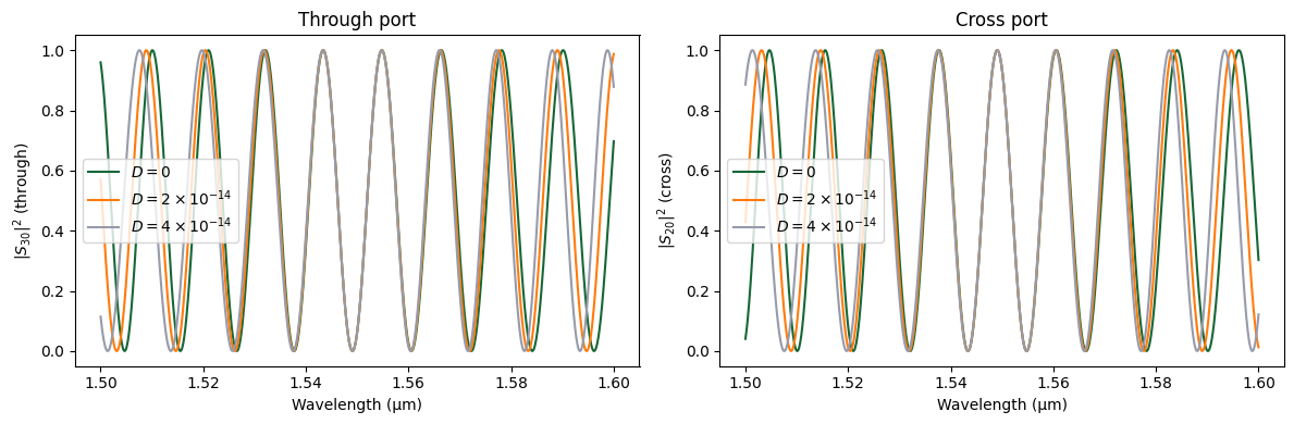
Dispersion curves the spectral envelope without degrading the peak extinction ratio. This effect becomes more pronounced for larger bandwidths and longer arm lengths.

Loss: Propagation Loss and Extra Loss

Each arm has independent loss parameters:

• Propagation loss \(L_p\) (dB/µm): scales with arm length.

• Extra loss \(L_0\) (dB): length-independent (e.g. bend loss in the arm).

Loss in the arms reduces the overall transmission and can also degrade the extinction ratio when the two arms have unequal loss.

fig, axes = plt.subplots(1, 2, figsize=(12, 4))

wavelengths = np.linspace(1.5, 1.6, 1001)

freqs = pf.C_0 / wavelengths

cases = [
    {
        "propagation_loss1": 0,
        "propagation_loss2": 0,
        "extra_loss1": 0,
        "extra_loss2": 0,
        "label": "Lossless",
    },
    {
        "propagation_loss1": 2e-3,
        "propagation_loss2": 2e-3,
        "extra_loss1": 0,
        "extra_loss2": 0,
        "label": "$L_p = 2$ dB/mm (both arms)",
    },
    {
        "propagation_loss1": 2e-3,
        "propagation_loss2": 5e-3,
        "extra_loss1": 0,
        "extra_loss2": 0,
        "label": "$L_{p1}=2$, $L_{p2}=5$ dB/mm",
    },
    {
        "propagation_loss1": 2e-3,
        "propagation_loss2": 2e-3,
        "extra_loss1": 0.5,
        "extra_loss2": 0,
        "label": "$L_p = 2$ dB/mm + $L_{0,1} = 0.5$ dB",
    },
]

for case in cases:
    model = pf.AnalyticMZIModel(
        n_eff1=2.4,
        n_eff2=2.4,
        n_group1=4.2,
        n_group2=4.2,
        length1=200,
        length2=230,
        propagation_loss1=case["propagation_loss1"],
        propagation_loss2=case["propagation_loss2"],
        extra_loss1=case["extra_loss1"],
        extra_loss2=case["extra_loss2"],
        reference_frequency=f0,
    )
    bb = model.black_box_component(port_spec="Strip")
    s = bb.s_matrix(freqs, show_progress=False)
    pn = sorted(s.ports)
    through_key = (f"{pn[0]}@0", f"{pn[3]}@0")
    cross_key = (f"{pn[0]}@0", f"{pn[2]}@0")

    axes[0].plot(
        wavelengths,
        10 * np.log10(np.abs(s[through_key]) ** 2 + 1e-30),
        label=case["label"],
    )
    axes[1].plot(
        wavelengths,
        10 * np.log10(np.abs(s[cross_key]) ** 2 + 1e-30),
        label=case["label"],
    )

for ax in axes:
    ax.set_xlabel("Wavelength (µm)")
    ax.set_ylim(-40, 1)

axes[0].set_ylabel("$|S_{31}|^2$ (dB)")
axes[0].set_title("Through port")
axes[0].legend(fontsize=8)

axes[1].set_ylabel("$|S_{41}|^2$ (dB)")
axes[1].set_title("Cross port")
axes[1].legend(fontsize=8)

fig.tight_layout()
plt.show()

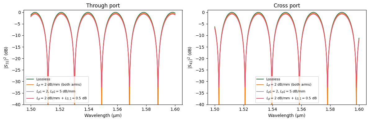
Symmetric loss (equal in both arms) reduces the overall transmission without degrading the extinction ratio. Asymmetric loss — whether from unequal propagation loss or extra loss in one arm — prevents perfect destructive interference, lifting the null floor and reducing the extinction ratio.

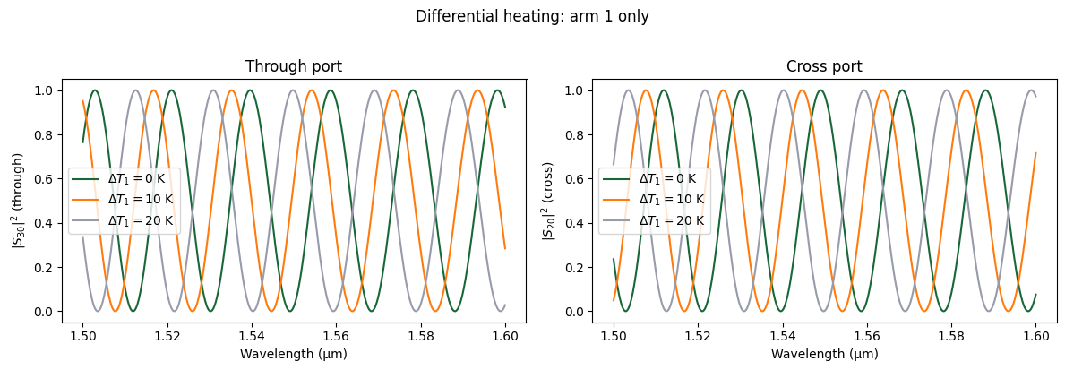
Temperature Sensitivity

Each arm has independent temperature parameters. A uniform temperature change shifts the spectral response, while a differential temperature between arms provides a powerful tuning mechanism.

For silicon waveguides, \(\mathrm{d}n/\mathrm{d}T \approx 1.8 \times 10^{-4}\;\text{K}^{-1}\). The temperature-induced phase shift is:

\[\Delta\phi_T \approx \frac{2\pi\,\ell}{c_0}\,\frac{\mathrm{d}n}{\mathrm{d}T}\,\Delta T\, f\]

Below we apply the same temperature change to both arms (uniform) and then to only one arm (differential).

Differential heating shifts the spectral response horizontally. This is the operating principle of thermo-optic MZI switches: by heating one arm, the interference condition shifts, allowing the switch to toggle between cross and through states.

T_ref = 293.0
dTs = [0, 10, 20]

fig, axes = plt.subplots(1, 2, figsize=(12, 4))
fig.suptitle("Differential heating: arm 1 only", y=1.02)

base_model = pf.AnalyticMZIModel(
    n_eff1=2.4,
    n_eff2=2.4,
    n_group1=4.2,
    n_group2=4.2,
    length1=200,
    length2=230,
    dn1_dT=1.8e-4,
    dn2_dT=1.8e-4,
    temperature1=T_ref,
    temperature2=T_ref,
    reference_temperature=T_ref,
    reference_frequency=f0,
)

bb = base_model.black_box_component(port_spec="Strip")

for dT in dTs:
    s = bb.s_matrix(
        freqs, model_kwargs={"temperature1": T_ref + dT}, show_progress=False
    )
    pn = sorted(s.ports)
    through_key = (f"{pn[0]}@0", f"{pn[3]}@0")
    cross_key = (f"{pn[0]}@0", f"{pn[2]}@0")

    label = f"$\\Delta T_1 = {dT}$ K"
    axes[0].plot(wavelengths, np.abs(s[through_key]) ** 2, label=label)
    axes[1].plot(wavelengths, np.abs(s[cross_key]) ** 2, label=label)

axes[0].set_xlabel("Wavelength (µm)")
axes[0].set_ylabel("$|S_{30}|^2$ (through)")
axes[0].set_title("Through port")
axes[0].legend()

axes[1].set_xlabel("Wavelength (µm)")
axes[1].set_ylabel("$|S_{20}|^2$ (cross)")
axes[1].set_title("Cross port")
axes[1].legend()

fig.tight_layout()
plt.show()

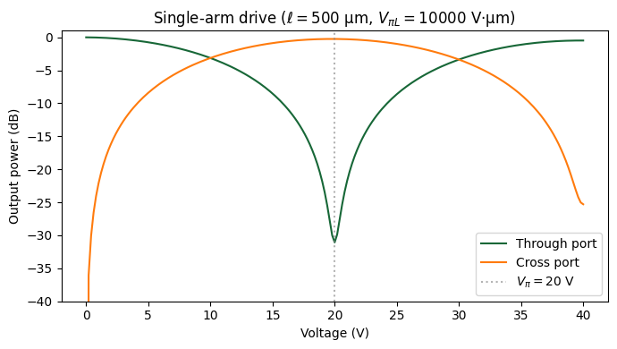
Electro-Optic MZI Modulator

The AnalyticMZIModel supports independent EO modulation of each arm through:

• \(V_{\pi L}\): Voltage-length product for a \(\pi\) phase shift in each arm.

• \(\mathrm{d}L/\mathrm{d}V\): Linear voltage-dependent loss.

• \(\mathrm{d}^2L/\mathrm{d}V^2\): Quadratic voltage-dependent loss.

Single-arm drive

In single-arm drive, voltage is applied to only one arm. The half-wave voltage is \(V_\pi = V_{\pi L} / \ell\).

At \(V = 0\), all power exits the cross port. At \(V = V_\pi\), the \(\pi\) phase shift switches power to the through port. Voltage-dependent loss (dloss_dv) prevents the cross port from reaching a perfect null at \(V_\pi\).

length_arm = 500
v_piL = 10000  # V·µm
v_pi = v_piL / length_arm

voltages = np.linspace(0, 2 * v_pi, 201)
f_center = np.array([f0])

through_power = []
cross_power = []

base_model = pf.AnalyticMZIModel(
    n_eff1=2.4,
    n_eff2=2.4,
    n_group1=4.2,
    n_group2=4.2,
    length1=length_arm,
    length2=length_arm,
    v_piL1=v_piL,
    dloss_dv_1=5e-5,
    voltage1=0,
    reference_frequency=f0,
)

bb = base_model.black_box_component(port_spec="Strip")

for V in voltages:
    s = bb.s_matrix(f_center, model_kwargs={"voltage1": V}, show_progress=False)
    pn = sorted(s.ports)
    through_key = (f"{pn[0]}@0", f"{pn[3]}@0")
    cross_key = (f"{pn[0]}@0", f"{pn[2]}@0")
    through_power.append(np.abs(s[through_key][0]) ** 2)
    cross_power.append(np.abs(s[cross_key][0]) ** 2)

through_power = np.array(through_power)
cross_power = np.array(cross_power)

fig, ax = plt.subplots(figsize=(7, 4))
ax.plot(voltages, 10 * np.log10(through_power + 1e-30), label="Through port")
ax.plot(voltages, 10 * np.log10(cross_power + 1e-30), label="Cross port")
ax.axvline(
    v_pi, color="gray", linestyle=":", alpha=0.6, label=f"$V_\\pi = {v_pi:.0f}$ V"
)
ax.set_xlabel("Voltage (V)")
ax.set_ylabel("Output power (dB)")
ax.set_title(
    f"Single-arm drive ($\\ell = {length_arm}$ µm, $V_{{\\pi L}} = {v_piL}$ V·µm)"
)
ax.set_ylim(-40, 1)
ax.legend()
fig.tight_layout()
plt.show()

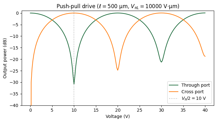
Push-pull drive

In push-pull configuration, opposite voltages are applied to the two arms (\(+V\) and \(-V\)). This halves the required drive voltage while maintaining a symmetric chirp. We can model this by setting \(V_{\pi L}\) on both arms and sweeping the voltage symmetrically.

Push-pull drive achieves the \(\pi\) phase shift with half the total voltage (\(V_{\pi,pp} = V_\pi / 2\)) compared to single-arm drive.

length_arm = 500
v_piL = 10000  # V·µm
v_pi = v_piL / length_arm

voltages = np.linspace(0, 2 * v_pi, 201)
f_center = np.array([f0])

through_power = []
cross_power = []

base_model = pf.AnalyticMZIModel(
    n_eff1=2.4,
    n_eff2=2.4,
    n_group1=4.2,
    n_group2=4.2,
    length1=length_arm,
    length2=length_arm,
    v_piL1=v_piL,
    v_piL2=v_piL,
    dloss_dv_1=5e-5,
    dloss_dv_2=5e-5,
    voltage1=0,
    voltage2=0,
    reference_frequency=f0,
)

bb = base_model.black_box_component(port_spec="Strip")

for V in voltages:
    s = bb.s_matrix(
        f_center, model_kwargs={"voltage1": V, "voltage2": -V}, show_progress=False
    )
    pn = sorted(s.ports)
    through_key = (f"{pn[0]}@0", f"{pn[3]}@0")
    cross_key = (f"{pn[0]}@0", f"{pn[2]}@0")
    through_power.append(np.abs(s[through_key][0]) ** 2)
    cross_power.append(np.abs(s[cross_key][0]) ** 2)

through_power = np.array(through_power)
cross_power = np.array(cross_power)

fig, ax = plt.subplots(figsize=(7, 4))
ax.plot(voltages, 10 * np.log10(through_power + 1e-30), label="Through port")
ax.plot(voltages, 10 * np.log10(cross_power + 1e-30), label="Cross port")
ax.axvline(
    v_pi / 2,
    color="gray",
    linestyle=":",
    alpha=0.6,
    label=f"$V_\\pi/2 = {v_pi/2:.0f}$ V",
)
ax.set_xlabel("Voltage (V)")
ax.set_ylabel("Output power (dB)")
ax.set_title(
    f"Push-pull drive ($\\ell = {length_arm}$ µm, $V_{{\\pi L}} = {v_piL}$ V·µm)"
)
ax.set_ylim(-40, 1)
ax.legend()
fig.tight_layout()
plt.show()

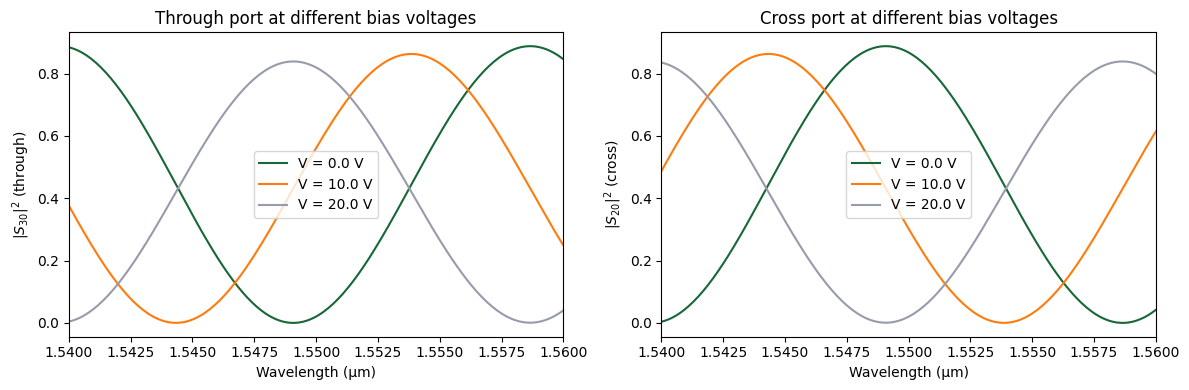
Spectral view at different bias voltages

Applying voltage shifts the entire spectral response.

model_eo = pf.AnalyticMZIModel(
    n_eff1=2.4,
    n_eff2=2.4,
    n_group1=4.2,
    n_group2=4.2,
    length1=length_arm,
    length2=length_arm + 30,
    propagation_loss1=1e-3,
    propagation_loss2=1e-3,
    v_piL1=v_piL,
    dloss_dv_1=5e-5,
    reference_frequency=f0,
)
bb_eo = model_eo.black_box_component(port_spec="Strip")

fig, axes = plt.subplots(1, 2, figsize=(12, 4))
for V in [0, v_pi / 2, v_pi]:
    s = bb_eo.s_matrix(freqs, model_kwargs={"voltage1": V}, show_progress=False)
    pn = sorted(s.ports)
    through_key = (f"{pn[0]}@0", f"{pn[3]}@0")
    cross_key = (f"{pn[0]}@0", f"{pn[2]}@0")
    axes[0].plot(wavelengths, np.abs(s[through_key]) ** 2, label=f"V = {V:.1f} V")
    axes[1].plot(wavelengths, np.abs(s[cross_key]) ** 2, label=f"V = {V:.1f} V")

axes[0].set_xlabel("Wavelength (µm)")
axes[0].set_ylabel("$|S_{30}|^2$ (through)")
axes[0].set_title("Through port at different bias voltages")
axes[0].set_xlim(1.54, 1.56)
axes[0].legend()

axes[1].set_xlabel("Wavelength (µm)")
axes[1].set_ylabel("$|S_{20}|^2$ (cross)")
axes[1].set_title("Cross port at different bias voltages")
axes[1].set_xlim(1.54, 1.56)
axes[1].legend()

fig.tight_layout()
plt.show()

Different Effective Indices Per Arm

In some designs the two arms have different waveguide cross-sections, resulting in different effective and group indices. The model supports this through n_eff2 and n_group2. When these are not set, they default to the arm-1 values.

Below we show how \(\Delta n_\text{eff}\) and \(\Delta n_\text{group}\) between arms shifts the spectral response, even with equal arm lengths.

spec1 = pf.PortSpec(
    description="500 nm Strip waveguide",
    width=2.25,
    limits=(-1, 1.22),
    num_modes=1,
    added_solver_modes=0,
    polarization="",
    target_neff=3.5,
    path_profiles=[(0.5, 0, (2, 0)), (2.5, 0, (1, 0))],
)
spec2 = pf.PortSpec(
    description="450 nm Strip waveguide",
    width=2.25,
    limits=(-1, 1.22),
    num_modes=1,
    added_solver_modes=0,
    polarization="",
    target_neff=3.5,
    path_profiles=[(0.45, 0, (2, 0)), (2.5, 0, (1, 0))],
)

opt_solver1 = pf.port_modes(
    spec1,
    [pf.C_0 / 1.55],
    mesh_refinement=40,
    group_index=True,
)

opt_solver2 = pf.port_modes(
    spec2,
    [pf.C_0 / 1.55],
    mesh_refinement=40,
    group_index=True,
)

n_eff1 = opt_solver1.data.n_eff.isel(mode_index=0, f=0).item()
n_group1 = opt_solver1.data.n_group.isel(mode_index=0, f=0).item()

n_eff2 = opt_solver2.data.n_eff.isel(mode_index=0, f=0).item()
n_group2 = opt_solver2.data.n_group.isel(mode_index=0, f=0).item()

mzi_model = pf.AnalyticMZIModel(
    n_eff1=n_eff1,
    n_eff2=n_eff2,
    n_group1=n_group1,
    n_group2=n_group2,
    length1=200,
    length2=200,
    reference_frequency=f0,
)

bb_mzi = mzi_model.black_box_component(port_spec="Strip")

_ = pf.plot_s_matrix(bb_mzi.s_matrix(freqs))

Progress: 100%
Progress: 100%
Progress: 100%

\(\Delta n_\text{eff}\) and \(\Delta n_\text{group}\) between arms act similarly to a length imbalance: it introduces a phase difference that creates spectral fringes.