Custom Model

PhotonForge provides a large number of models, particularly for passive optical devices. However, custom models can be easily implemented for specific use-cases. This short guide provides an example of custom model implementation for a voltage-controlled phase-shifter, that could be used in the Tunable MZI and the Switch Array examples.
The phase-shifter is based on a WaveguideModel with propagation index modeled as:
in which \(V\) is the applied voltage, \(\gamma\) is a coefficient that relates the variation of the index with the squared voltage.
This model could be applied to a thermo-optic phase-shifter, where the temperature in the thermal element is proportional to the input electrical power (thus squared voltage) and the coefficient depends on the overall geometry and materials. It can be calculated using a heat simulation, but we will skip that step to keep this guide short.
Any custom model must be derived from the base Model class and implement the start method. This guide will implement it alongside a proper __init__ to provide a full reference for other models, but the source code for all PhotonForge models is also available in our docs.
[1]:
import numpy as np
import photonforge as pf
Class initialization
The __init__ method must call super().__init__ with all user-provided arguments. That ensures the parametric_kwargs attribute of all instances is properly initialized, and they can be later used as parametric models and updated when necessary.
During circuit simulations or Monte Carlo runs, models can be updated (for example, through the updates parameter in CircuitModel.start). When that happens, the model is recreated from its (updated) parametric keyword arguments, so any changes to the model made after creation are lost. That means that model state should only be set
in the __init__ method.
Here’s what NOT to do:
[2]:
class BadModel(pf.Model):
    def __init__(self, a=0, b=1):
        super().__init__(a=a)  # ERROR: missing parameter b
        self.a = a
        self.b = b
        self.abc = 0

    def set_c(self, c):
        self.abc = self.a * self.b * c  # ERROR: this change will vanish after update

    def start(self):
        pass


bad_model = BadModel(a=1, b=2)

print(f"Note the missing parameter 'b': {bad_model.parametric_kwargs=}")
Note the missing parameter 'b': bad_model.parametric_kwargs={'a': 1}
[3]:
bad_model.set_c(3)

print(f"""New model state {bad_model.abc=}
But no changes in the 'parametric_kwargs' dictionary: {bad_model.parametric_kwargs=}""")
New model state bad_model.abc=6
But no changes in the 'parametric_kwargs' dictionary: bad_model.parametric_kwargs={'a': 1}
[4]:
bad_model.update(a=10)

print(f"""Updated parameter 'a': {bad_model.a=}
Parameter 'b' should not be updated, but lost its original value (2): {bad_model.b=}
Call to 'set_c' forgotten: {bad_model.abc=}""")
Updated parameter 'a': bad_model.a=10
Parameter 'b' should not be updated, but lost its original value (2): bad_model.b=1
Call to 'set_c' forgotten: bad_model.abc=0
A better way to implement the same model would be to remove the state change from outside the __init__ method, and refactor the internal state as a property calculated when needed:
[5]:
class GoodModel(pf.Model):
    def __init__(self, a=0, b=0, c=0):
        super().__init__(a=a, b=b, c=c)  # All state as __init__ arguments

    @property
    def abc(self):
        p = self.parametric_kwargs
        return p["a"] * p["b"] * p["c"]

    def start(self):
        pass


good_model = GoodModel(a=1, b=2)
print(f"All paramters properly initialized: {good_model.parametric_kwargs=}")

# Use update to set new value
good_model.update(c=3)
print(f"""Updated 'parametric_kwargs' dictionary: {good_model.parametric_kwargs}
New model state {good_model.abc=}""")

good_model.update(a=10)
print(f"""Updated 'parametric_kwargs' dictionary: {good_model.parametric_kwargs}
New model state {good_model.abc=}""")
All paramters properly initialized: good_model.parametric_kwargs={'a': 1, 'b': 2, 'c': 0}
Updated 'parametric_kwargs' dictionary: {'a': 1, 'b': 2, 'c': 3}
New model state good_model.abc=6
Updated 'parametric_kwargs' dictionary: {'a': 10, 'b': 2, 'c': 3}
New model state good_model.abc=60
S-matrix computation
We must provide a way for our custom model to actually compute the S matrix for a given component. That is done in the start method.
The start method will receive keyword arguments passed to call to the model or component s_matrix method through the model_kwargs argument. For this model, we want to accept a voltage value that overrides the internal voltage and allows us to set it dynamically.
For this model, we will leverage the existing WaveguideModel to perform the actual computation based on the calculated propagation constant.
Alternatively, we could perform the computation in the function itself and return the resulting SMatrix. If the computation is a long process, the start method can be used to simply kick it off and return an object that can be used to monitor the computation progress, but that will be left for another guide.
Full implemetation
Putting it all together, we have the following implementation.
It is paramount to register the custom model class after creating it, otherwise PhotonForge won’t be able to use it automatically.
[6]:
class ThermalModel(pf.Model):
    def __init__(self, n_complex, voltage=0, coefficient=3e-4):
        super().__init__(
            n_complex=n_complex,
            voltage=voltage,
            coefficient=coefficient,
        )

    @pf.cache_s_matrix
    def start(self, component, frequencies, voltage=None, **kwargs):
        p = self.parametric_kwargs

        # Use voltage as an `s_matrix` kwarg, but fallack to default value
        if voltage is None:
            voltage = p["voltage"]

        # Main model equation
        n_complex = p["n_complex"] + p["coefficient"] * voltage**2

        # Auxiliary model for the computation
        wg_model = pf.WaveguideModel(n_complex)
        return wg_model.start(component, frequencies, **kwargs)


pf.register_model_class(ThermalModel)
Usage Example: Tunable Microring Resonator
We start by configuring the simulation environment
We assign the basic photonforge technology to
pf.config.default_technology.We define default keyword arguments for our components, specifying a
"Strip"port and a radius of10.We define the wavelength range.
[7]:
import matplotlib.pyplot as plt
from photonforge.live_viewer import LiveViewer

viewer = LiveViewer()

# Set default technology to the basic technology provided by photonforge
pf.config.default_technology = pf.basic_technology()

# Set default keyword arguments for simulations: use Strip port specification and radius of 10
pf.config.default_kwargs = {"port_spec": "Strip", "radius": 10}

# Define wavelength range for the simulation (in micrometers)
wavelengths = np.linspace(1.546, 1.548, 201)

# Convert wavelengths to frequencies (Hz) using speed of light constant
frequencies = pf.C_0 / wavelengths
LiveViewer started at http://localhost:33417
Coupler Definition
We now define the directional coupler that will be used to couple light into and out of the microring:
We create a dual-ring directional coupler with a waveguide gap of
0.9 µmand a coupling region length of10 µm.We set the
Tidy3Dgrid specification to12to reduce simulation cost but with reasonable accuracy.
[8]:
# Set the coupling length for the directional coupler
coupling_length = 10

# Define a dual-ring directional coupler with specified geometry and waveguide spacing
dc_coupler = pf.parametric.ring_coupler(
    coupling_distance=0.9,  # distance between the coupled waveguides (µm)
    coupling_length=coupling_length,  # coupling region length (µm)
    model=pf.Tidy3DModel(grid_spec=12),
)

# Display the coupler layout
viewer(dc_coupler)
[8]:

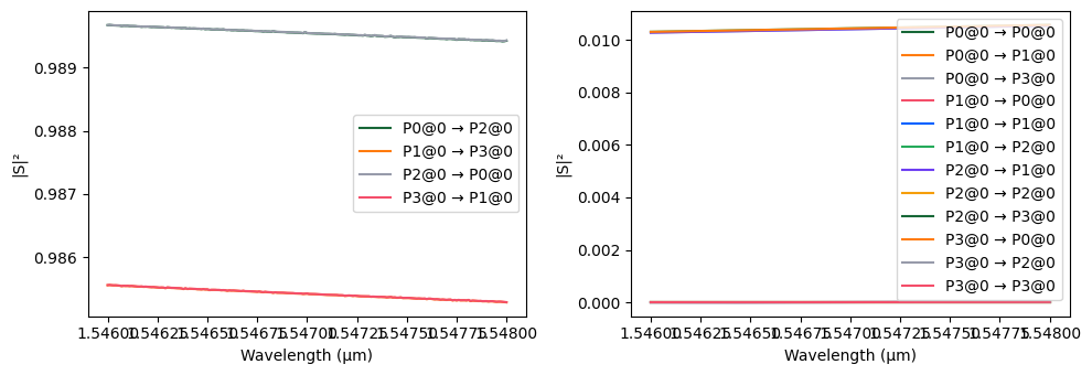
The coupler has been designed to achieve approximately 1% power coupling between the waveguides. We simulate the S-matrix of the directional coupler over the defined frequency range. The resulting plot confirms the low coupling regime, with around 1% of power transferred between ports.
[9]:
# Compute the S-matrix of the dual-ring coupler over the specified frequencies
s_matrix_dc = dc_coupler.s_matrix(frequencies)
_ = pf.plot_s_matrix(s_matrix_dc)
Uploading task 'P0@0…'
Uploading task 'P1@0…'
Uploading task 'P2@0…'
Uploading task 'P3@0…'
Starting task 'P1@0': https://tidy3d.simulation.cloud/workbench?taskId=fdve-bb4de2fe-a1b9-4e8c-82c9-5f87dcf59654
Starting task 'P0@0': https://tidy3d.simulation.cloud/workbench?taskId=fdve-a962f015-c198-4954-9ec8-6a40c033fce2
Downloading data from 'P1@0'…
Starting task 'P2@0': https://tidy3d.simulation.cloud/workbench?taskId=fdve-35992f81-6e05-49c8-89d6-b632d0cd52e9
Starting task 'P3@0': https://tidy3d.simulation.cloud/workbench?taskId=fdve-3cfeae5e-a7bc-44a7-86a0-70e223a1eaf7
Downloading data from 'P0@0'…
Downloading data from 'P2@0'…
Downloading data from 'P3@0'…
Progress: 100%
Waveguide with Thermal Model
Next, we define the straight waveguide section and place a metal heater on top:
We use a propagation loss, converted to an imaginary part of the refractive index (
kappa) for accurate modeling.A heater is designed using a tapered metal path, consisting of wide pads and a narrow central section.
This heater is positioned on top of the waveguide.
We solve the port mode to get the base complex index and add loss by modifying the imaginary part.
A custom
ThermalModelis instantiated with this lossy refractive index, and added to the waveguide.Finally, we visualize the structure including the integrated heater.
[10]:
# Set propagation loss in dB/cm
alpha = 10

# Define metal heater geometry
heater_width = 5
pad_width = 20
transition_length = 10

# Calculate imaginary part of refractive index due to propagation loss
kappa = (alpha * wavelengths * 1e-4 * np.log(10)) / (40 * np.pi)

# Create the waveguide geometry with length equal to the coupler
wg = pf.parametric.straight(length=coupling_length)

# Define the heater path with tapered metal pads and narrow central section
heater = (
    pf.Path((-2 * transition_length - pad_width, 0), pad_width)
    .segment((-2 * transition_length, 0), pad_width)
    .segment((-transition_length, 0), heater_width)
    .segment((coupling_length + transition_length, 0))
    .segment((coupling_length + 2 * transition_length, 0), pad_width)
    .segment((coupling_length + 2 * transition_length + pad_width, 0), pad_width)
)

# Attach the metal heater to the waveguide
wg.add((5, 0), heater)

# Solve for the port mode of the waveguide and extract the complex refractive index
mode_solver = pf.port_modes(port=wg.ports["P0"], frequencies=frequencies)
n_complex = mode_solver.data.n_complex.values.T + 1j * kappa  # add propagation loss

# Instantiate a thermal model using the lossy index
thermal_model = ThermalModel(n_complex=n_complex)

# Attach the thermal model to the waveguide
wg.add_model(thermal_model, "Thermal")

# Visualize the waveguide and heater
viewer(wg)
Uploading task 'Mode-ModeSolver…'Progress: 0% -
Starting task 'Mode-ModeSolver': https://tidy3d.simulation.cloud/workbench?taskId=mo-c0266d52-f01c-49da-9db7-a7c53c16f74b
Downloading data from 'Mode-ModeSolver'…
Progress: 100%
[10]:

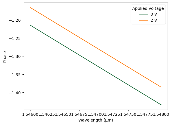
Before assembling the full circuit, we test the thermal model directly on the waveguide. We compute the S-matrix at 0 V and 2 V to observe the phase change. The phase shift of the S21 response is plotted as a function of wavelength. This confirms that the custom thermal model applies a voltage-dependent phase shift, as expected.
[11]:
# Compute S-matrix for the waveguide with no voltage applied
s_v0 = wg.s_matrix(frequencies)

# Compute S-matrix with 2 V applied to the thermal model
s_v2 = wg.s_matrix(frequencies, model_kwargs={"voltage": 2})

# Plot the phase response (angle of S21) for both voltages
plt.plot(wavelengths, np.angle(s_v0[("P0@0", "P1@0")]), label="0 V")
plt.plot(wavelengths, np.angle(s_v2[("P0@0", "P1@0")]), label="2 V")

# Label the axes
plt.xlabel("Wavelength (µm)")
plt.ylabel("Phase")

# Add legend to differentiate voltage levels
plt.legend(title="Applied voltage")

# Display the plot
plt.show()
Progress: 100%
Progress: 100%
To ensure consistency across the layout, we also assign the same lossy refractive index to a waveguide bend:
[12]:
# Create a bend waveguide using default parameters
bend = pf.parametric.bend(model=pf.WaveguideModel(n_complex=n_complex))

# Visualize the bend structure
viewer(bend)
[12]:

Tunable Microring Resonator Construction
We now build a tunable microring resonator by connecting the previously defined components:
The
netlistdefines each component: a directional coupler (dc), a phase shifter (ps), and two bends (b0andb1).These components are connected in a loop to form the microring structure.
External ports are exposed on the input and output sides of the directional coupler.
A
CircuitModelis assigned to handle simulation of the entire system.Finally, we use
component_from_netlistto construct the full microring resonator.
[13]:
# Define the netlist for a tunable microring resonator
netlist_mrr = {
    "name": "Tunable Microring Resonator",  # name of the component
    "instances": {
        "dc": dc_coupler,  # directional coupler
        "ps": wg,  # waveguide with heater (phase shifter)
        "b0": bend,
        "b1": bend,
    },
    # Define how components are connected
    "connections": [
        (("b0", "P1"), ("dc", "P1")),  # connect top bend to one side of the coupler
        (("b1", "P0"), ("dc", "P3")),  # connect bottom bend to the other side
        (("ps", "P0"), ("b0", "P0")),  # connect phase shifter to top bend
    ],
    # Define external ports (input and output)
    "ports": [("dc", "P0"), ("dc", "P2")],
    # Assign a CircuitModel to simulate the entire microring
    "models": [(pf.CircuitModel(), "Circuit")],
}

# Build the microring resonator from the netlist
mrr = pf.component_from_netlist(netlist_mrr)

# Visualize the resulting component
viewer(mrr)
[13]:

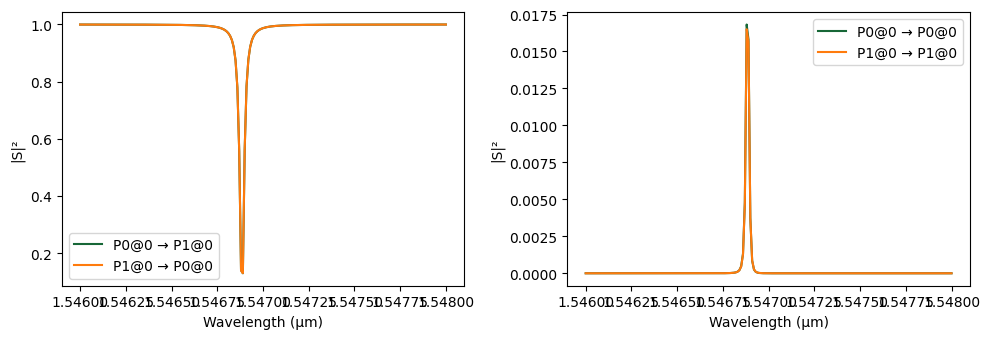
[14]:
# Compute the S-matrix of the full circuit
s_matrix = mrr.s_matrix(frequencies)

# Plot transmission
fig, ax = pf.plot_s_matrix(s_matrix)
Uploading task 'Mode-Stripwaveguide…'
Uploading task 'Mode-Stripwaveguide…'
Uploading task 'Mode-Stripwaveguide…'
Uploading task 'Mode-Stripwaveguide…'
Starting task 'Mode-Stripwaveguide': https://tidy3d.simulation.cloud/workbench?taskId=mo-7b365e99-269b-40c2-bbf2-92e92d01cc07
Starting task 'Mode-Stripwaveguide': https://tidy3d.simulation.cloud/workbench?taskId=mo-3f9491c5-3810-4bd3-b77c-31590fa522f3
Starting task 'Mode-Stripwaveguide': https://tidy3d.simulation.cloud/workbench?taskId=mo-e7c83762-13ce-4e8f-b47e-240d9ae25471
Downloading data from 'Mode-Stripwaveguide'…
Downloading data from 'Mode-Stripwaveguide'…
Downloading data from 'Mode-Stripwaveguide'…
Starting task 'Mode-Stripwaveguide': https://tidy3d.simulation.cloud/workbench?taskId=mo-85110b98-c2e3-4798-943f-bae1dcccc073
Downloading data from 'Mode-Stripwaveguide'…
Progress: 100%
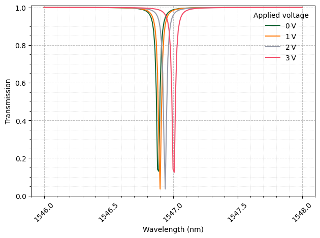
Resonance Tuning via Applied Voltage
To observe how the microring’s resonance shifts under different voltages:
We sweep the applied voltage across the waveguide heater with values of
0 V,2 V, and3 V.For each voltage, we simulate the S-matrix and extract the transmission (
S21).The transmission spectra are plotted against wavelength in nanometers.
The resonance shift is clearly visible, confirming the thermo-optic tuning effect of the microring.
💡 Reference indexing: When updating model parameters during S-matrix simulation, we use the syntax
(component_name, reference_index). This allows precise control when the same component appears multiple times within a larger layout. For example,(wg.name, 0)refers to the first reference of thewgcomponent inside themrr. If there were multiple uses ofwg, we could address and update each independently by changing the index.
[15]:
import matplotlib.ticker as ticker

# the list of voltages
voltages = [0, 1, 2, 3]

# make one figure/axes
fig, ax = plt.subplots()

for v in voltages:
    updates = {(wg.name, 0): {"model_updates": {"voltage": v}}}
    s_matrix = mrr.s_matrix(frequencies, model_kwargs={"updates": updates})
    s21 = s_matrix[("P0@0", "P1@0")]
    ax.plot(
        wavelengths * 1e3,
        np.abs(s21) ** 2,
        label=f"{v} V",
        linewidth=1.5,
    )

# labels & legend
ax.set_xlabel("Wavelength (nm)")
ax.set_ylabel("Transmission")
ax.set_ylim(0, 1.01)
ax.legend(title="Applied voltage", loc="upper right", frameon=False)

# major ticks every 0.5 nm, minor ticks every 0.1 nm
ax.xaxis.set_major_locator(ticker.MultipleLocator(0.5))
ax.xaxis.set_minor_locator(ticker.MultipleLocator(0.1))
ax.xaxis.set_major_formatter(ticker.FormatStrFormatter("%.1f"))

# y‑axis major ticks every 0.2, minor every 0.05
ax.yaxis.set_major_locator(ticker.MultipleLocator(0.2))
ax.yaxis.set_minor_locator(ticker.MultipleLocator(0.05))

# enable both major & minor gridlines
ax.grid(which="major", linestyle="--", linewidth=0.7, alpha=0.8)
ax.grid(which="minor", linestyle=":", linewidth=0.5, alpha=0.5)

# rotate x‑labels for readability
plt.setp(ax.get_xticklabels(which="major"), rotation=45)

plt.tight_layout()
plt.show()
Progress: 100%
Progress: 100%
Progress: 100%
Progress: 100%