
Cascaded Rings Filter

In this example, we will use a combination of component-level FDTD simulations and circuit simulations to build a filter based on cascaded ring resonators. They can be use to tailor the resonance spectra of a ring filter to make it flatter near the pass band as well as make the roll-off steeper in the rejection band. More details about ring-based filters can be found in [1].
References
Geuzebroek, D.H., Driessen, A. (2006). “Ring-Resonator-Based Wavelength Filters.” In: Venghaus, H. (eds) Wavelength Filters in Fibre Optics. Springer Series in Optical Sciences, vol 123. Springer, Berlin, Heidelberg. DOI: 10.1007/3-540-31770-8_9.
[1]:
import pathlib

import matplotlib.pyplot as plt
import numpy as np
import photonforge as pf
import siepic_forge as siepic
import tidy3d as td
For the design, we will will use the SiEPIC OpenEBL technology and the its predefined strip waveguide for TE mode in the C band.
[2]:
tech = siepic.ebeam()
pf.config.default_technology = tech

print("Predefined waveguide profiles: " + ", ".join(tech.ports))
Predefined waveguide profiles: MM_TE_1550_2000, MM_TE_1550_3000, Rib_TE_1310_350, Rib_TE_1550_500, Slot_TE_1550_500, TE-TM_1550_450, TE_1310_350, TE_1310_410, TE_1550_500, TM_1310_350, TM_1550_500, eskid_TE_1550
[3]:
wavelengths = np.linspace(1.548, 1.552, 81)
port_spec = tech.ports["TE_1550_500"]
Point Couplers
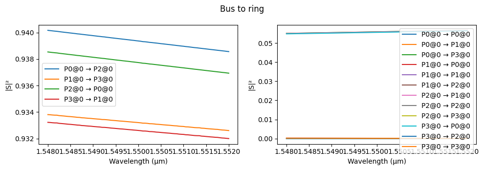
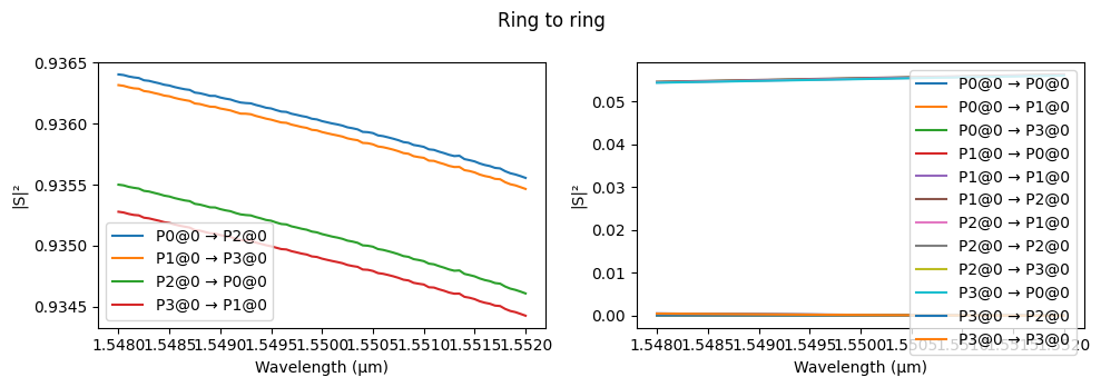
Instead of solving the full cascaded problem in FDTD, we can solve for the two point couplers (i.e. coupling between the bus waveguide to ring waveguide and coupling between two ring waveguides). Then, we will be able to utilize the computed S matrix to dynamically vary the number of rings and run fast circuit simulations.
We use parametric components to quickly design both couplers:
ring_coupler for the bus, and
dual_ring_coupler for the inter-ring coupling.
Note that we decrease the default mesh refinement from 20 to 15 minimal grid cells per wavelength to decrease the simulation size. That can slightly change the exact resonant frequencies of the filter, but fabrication imperfections usually have a much higher impact here, so that is not so important in this example.
However, we define a smaller shut-off condition (10⁻⁷, instead of the default 10⁻⁵) to decrease residual fields in the simulation, and we increase the default run time quality factor to ensure enough time for the shut-off condition. These measures are necessary because we will combine the frequency-domain S parameters into resonant devices, where small numerical errors can be amplified and lead to non-passive responses (identifiable, for example, if we see any S parameter magnitude above unit).
[4]:
pf.config.default_mesh_refinement = 15

# Default parameters for parametric components
pf.config.default_kwargs = {
    "port_spec": port_spec,
    "radius": 10,
    "coupling_distance": 0.6,  # measured between waveguide centers
    "tidy3d": {
        "run_time": td.RunTimeSpec(quality_factor=10),
        "shutoff": 1e-7,
    },
}
[5]:
bus_to_ring = pf.parametric.s_bend_ring_coupler(s_bend_offset=port_spec.width)
bus_to_ring
[5]:

[6]:
ring_to_ring = pf.parametric.dual_ring_coupler()
ring_to_ring
[6]:

We will run the S parameter simulation and plot it with our S matrix plot utility for both couplers.
[7]:
fig, _ = pf.plot_s_matrix(bus_to_ring.s_matrix(pf.C_0 / wavelengths))
fig.suptitle("Bus to ring")

fig, _ = pf.plot_s_matrix(ring_to_ring.s_matrix(pf.C_0 / wavelengths))
_ = fig.suptitle("Ring to ring")
Starting…
22:35:54 -03 Loading simulation from local cache. View cached task using web UI
             at
             'https://tidy3d.simulation.cloud/workbench?taskId=mo-4a2a9595-7e94-
             454f-8d00-c66bf305ad85'.
             Loading simulation from local cache. View cached task using web UI
             at
             'https://tidy3d.simulation.cloud/workbench?taskId=mo-cd7a9499-0b25-
             4a89-a1c1-c119a3cd415b'.
             Loading simulation from local cache. View cached task using web UI
             at
             'https://tidy3d.simulation.cloud/workbench?taskId=fdve-4d69d724-871
             6-4b0d-9a8f-86192513039a'.
             WARNING: Warning messages were found in the solver log. For more
             information, check 'SimulationData.log' or use
             'web.download_log(task_id)'.
             Loading simulation from local cache. View cached task using web UI
             at
             'https://tidy3d.simulation.cloud/workbench?taskId=fdve-84ba1b28-d8a
             9-4444-b025-20ffc498927e'.
             Loading simulation from local cache. View cached task using web UI
             at
             'https://tidy3d.simulation.cloud/workbench?taskId=mo-3d222609-bb58-
             4cc6-a2a8-add60412a123'.
22:35:55 -03 Loading simulation from local cache. View cached task using web UI
             at
             'https://tidy3d.simulation.cloud/workbench?taskId=mo-d303ddde-be1c-
             43d9-a8ad-ef79d3bb0b28'.
             Loading simulation from local cache. View cached task using web UI
             at
             'https://tidy3d.simulation.cloud/workbench?taskId=fdve-4fed27dd-cff
             3-4ae5-b171-f6fd95287c1f'.
             WARNING: Warning messages were found in the solver log. For more
             information, check 'SimulationData.log' or use
             'web.download_log(task_id)'.
             Loading simulation from local cache. View cached task using web UI
             at
             'https://tidy3d.simulation.cloud/workbench?taskId=fdve-9f019dc5-13b
             5-4a91-91e1-bad84d42ee8d'.
             Loading simulation from local cache. View cached task using web UI
             at
             'https://tidy3d.simulation.cloud/workbench?taskId=fdve-ca153514-d51
             d-4a17-b1fd-d03da125764a'.
             Loading simulation from local cache. View cached task using web UI
             at
             'https://tidy3d.simulation.cloud/workbench?taskId=fdve-9b19b0d9-65d
             7-4483-b588-92c714dffb5d'.
             Loading simulation from local cache. View cached task using web UI
             at
             'https://tidy3d.simulation.cloud/workbench?taskId=fdve-0bc2cc98-4f5
             2-480f-bbca-f3d26feb716e'.
             Loading simulation from local cache. View cached task using web UI
             at
             'https://tidy3d.simulation.cloud/workbench?taskId=fdve-ea6097d5-c52
             e-4158-8d11-b08ffbcc7a97'.
Progress: 100%
Starting…
22:35:57 -03 Loading simulation from local cache. View cached task using web UI
             at
             'https://tidy3d.simulation.cloud/workbench?taskId=fdve-95a51b11-0b1
             1-4e3c-a685-1e5d15e5f228'.
             Loading simulation from local cache. View cached task using web UI
             at
             'https://tidy3d.simulation.cloud/workbench?taskId=fdve-214a5af9-770
             6-49ac-8c5c-6fc89da7b9df'.
             Loading simulation from local cache. View cached task using web UI
             at
             'https://tidy3d.simulation.cloud/workbench?taskId=fdve-a6194a33-d3c
             9-444a-befd-60002b254c59'.
             WARNING: Warning messages were found in the solver log. For more
             information, check 'SimulationData.log' or use
             'web.download_log(task_id)'.
             Loading simulation from local cache. View cached task using web UI
             at
             'https://tidy3d.simulation.cloud/workbench?taskId=fdve-0d234180-668
             2-4be8-941f-e0a035152e6f'.
             Loading simulation from local cache. View cached task using web UI
             at
             'https://tidy3d.simulation.cloud/workbench?taskId=fdve-d36efc4f-642
             6-4fcf-ae8c-b663cd19595f'.
             Loading simulation from local cache. View cached task using web UI
             at
             'https://tidy3d.simulation.cloud/workbench?taskId=fdve-53f425c5-8a1
             a-4878-83ee-e819ca7a256d'.
22:35:58 -03 Loading simulation from local cache. View cached task using web UI
             at
             'https://tidy3d.simulation.cloud/workbench?taskId=fdve-eb88efe5-28a
             2-4b7d-8c33-edea6da7d346'.
             WARNING: Warning messages were found in the solver log. For more
             information, check 'SimulationData.log' or use
             'web.download_log(task_id)'.
             Loading simulation from local cache. View cached task using web UI
             at
             'https://tidy3d.simulation.cloud/workbench?taskId=fdve-3e6d31da-2fc
             9-4052-ac9f-0ac18da99b4f'.
             Loading simulation from local cache. View cached task using web UI
             at
             'https://tidy3d.simulation.cloud/workbench?taskId=fdve-8ebfd675-e69
             b-4310-9a66-2402f179b1a7'.
             Loading simulation from local cache. View cached task using web UI
             at
             'https://tidy3d.simulation.cloud/workbench?taskId=fdve-6cab7af9-4be
             8-4f4d-9be9-0eea86571d4d'.
22:35:59 -03 Loading simulation from local cache. View cached task using web UI
             at
             'https://tidy3d.simulation.cloud/workbench?taskId=fdve-f7ab855c-554
             d-4f39-8502-4b1f3c560d73'.
             Loading simulation from local cache. View cached task using web UI
             at
             'https://tidy3d.simulation.cloud/workbench?taskId=fdve-51bab9a6-47e
             3-4bbb-8289-45faaee6e1b4'.
Progress: 100%
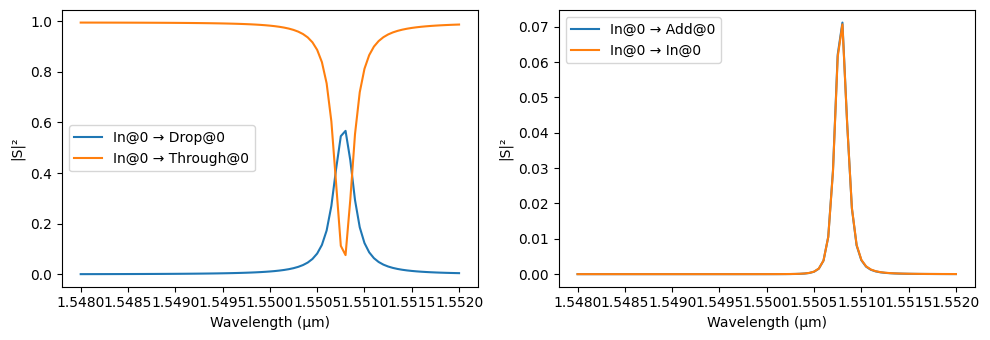
Add drop filter
Now that we have simulated S parameters for the point couplers, we use a netlist-driven layout to create an add-drop filter and look at the resonant response of the ring. The component_from_netlist function can be used to build an add-drop filter component with a circuit model.
[8]:
netlist_add_drop = {
    "name": "add_drop",
    "instances": [bus_to_ring, bus_to_ring],
    "connections": [((1, "P1"), (0, "P3"))],
    "ports": [
        (0, "P0", "In"),
        (0, "P2", "Through"),
        (1, "P0", "Add"),
        (1, "P2", "Drop"),
    ],
    "models": [pf.CircuitModel()],
}

add_drop = pf.component_from_netlist(netlist_add_drop)
add_drop
[8]:

Since we have added a Circuit model to the add-drop filter, PhotonForge automatically uses the S parameters that were already calculated for the instance components to calculate the circuit’s S matrix. It will need to perform a few mode-solver calculations to make sure the correct phases are accounted for after instance rotations.
[9]:
s_matrix_add_drop = add_drop.s_matrix(frequencies=pf.C_0 / wavelengths)
_ = pf.plot_s_matrix(s_matrix_add_drop, input_ports=["In"])
Starting…
22:36:00 -03 Loading simulation from local cache. View cached task using web UI
             at
             'https://tidy3d.simulation.cloud/workbench?taskId=mo-926663ad-4cda-
             4690-9c35-b5fe278b9444'.
             Loading simulation from local cache. View cached task using web UI
             at
             'https://tidy3d.simulation.cloud/workbench?taskId=mo-3b8ee5b9-0e19-
             41be-99a1-ff2dc1fecca2'.
             Loading simulation from local cache. View cached task using web UI
             at
             'https://tidy3d.simulation.cloud/workbench?taskId=mo-94ed0160-dc5a-
             463d-be8c-82170a082bf6'.
             Loading simulation from local cache. View cached task using web UI
             at
             'https://tidy3d.simulation.cloud/workbench?taskId=mo-e84ca97d-3210-
             4086-b3fc-a64e437a62a6'.
Progress: 100%
Coupled Rings
Next, we can create a coupled-ring filter to see the effect of cascading identical resonators. Again, we will use netlist helper to create the component.
[10]:
netlist_coupled_rings = {
    "name": "cascaded_ring_filter",
    "instances": {
        "bus_coupler0": bus_to_ring,
        "bus_coupler1": bus_to_ring,
        "ring_coupler0": ring_to_ring,
        "ring_coupler1": ring_to_ring,
    },
    "connections": [
        (("ring_coupler0", "P0"), ("bus_coupler0", "P1")),
        (("ring_coupler1", "P0"), ("ring_coupler0", "P1")),
        (("bus_coupler1", "P3"), ("ring_coupler1", "P1")),
    ],
    "ports": [
        ("bus_coupler0", "P0", "In"),
        ("bus_coupler1", "P2", "Drop"),
        ("bus_coupler0", "P2", "Through"),
        ("bus_coupler1", "P0", "Add"),
    ],
    "models": [pf.CircuitModel()],
}


coupled_rings = pf.component_from_netlist(netlist_coupled_rings)
coupled_rings
[10]:

[11]:
s_matrix_coupled_rings = coupled_rings.s_matrix(frequencies=pf.C_0 / wavelengths)
_ = pf.plot_s_matrix(s_matrix_coupled_rings, input_ports=["In"])
Progress: 100%
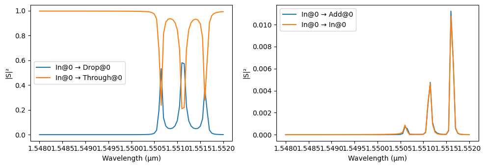
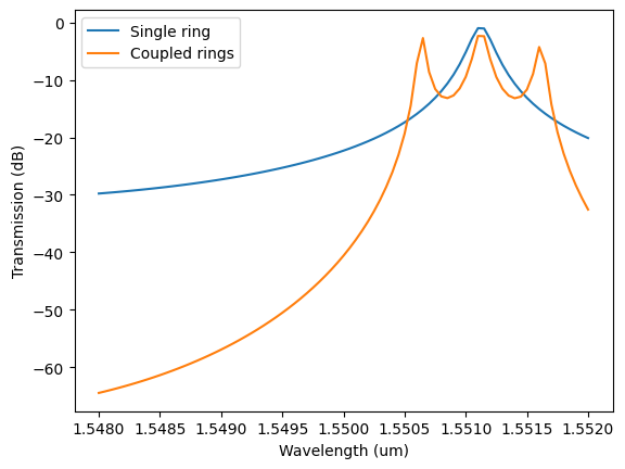
We can see how it is possible to change the filter response not just at the pass band but also modify it to achieve a sharp roll-off in the rejection band.
[12]:
plt.plot(
    wavelengths,
    20 * np.log10(np.abs(s_matrix_add_drop[(f"In@0", f"Drop@0")])),
    label=f"Single ring",
)
plt.plot(
    wavelengths,
    20 * np.log10(np.abs(s_matrix_coupled_rings[(f"In@0", f"Drop@0")])),
    label=f"Coupled rings",
)
plt.xlabel("Wavelength (um)")
plt.ylabel("Transmission (dB)")
_ = plt.legend()
Cascaded add-drop filters
Another common configuration is to cascade the rings in series in the same bus waveguide, possibly with slightly different resonant frequencies. We will use a termination on one of the add/drop filter ports and connect a routing waveguide bend to the other, which can be used to connect to other parts of the circuit later.
We start by creating the termination (from scratch) and the bend (using a parametric component):
[13]:
termination = pf.Component("Termination")
termination.add("Si", pf.stencil.linear_taper(20, (0.5, 0.1)))
termination.add_port(pf.Port((0, 0), 0, port_spec))
termination.add_model(pf.Tidy3DModel())
termination
[13]:

[14]:
bend = pf.parametric.bend(name="Bend")
bend
[14]:

Now we create the terminated single add/drop filter as a parametric component, using an extra straight section in the ring to change the resonant frequency. Because of the simplicity of this component, we can still use a netlist-driven design.
[15]:
@pf.parametric_component
def create_add_drop(*, added_length=0):
    # Basic add-drop filter netlist
    netlist = {
        "instances": {
            "bus_coupler0": bus_to_ring,
            "bus_coupler1": bus_to_ring,
            "bend0": bend,
            "bend1": bend,
            "termination": termination,
        },
        "connections": [
            (("bus_coupler1", "P1"), ("bus_coupler0", "P3")),
            (("bend1", "P0"), ("bus_coupler1", "P0")),
            (("termination", "P0"), ("bend1", "P1")),
            (("bend0", "P1"), ("bus_coupler1", "P2")),
        ],
        "ports": [
            ("bus_coupler0", "P0"),
            ("bus_coupler0", "P2"),
            ("bend0", "P0", "Add/Drop"),
        ],
        "models": [pf.CircuitModel()],
    }

    if added_length > 0:
        # If we need extra length, add 2 spacer instances to the netlist and
        # re-connect the instances appropriately
        spacer = pf.parametric.straight(length=added_length)
        netlist["instances"]["spacer0"] = spacer
        netlist["instances"]["spacer1"] = spacer

        netlist["connections"] = [
            (("spacer0", "P0"), ("bus_coupler0", "P1")),
            (("spacer1", "P1"), ("bus_coupler0", "P3")),
            (("bus_coupler1", "P1"), ("spacer1", "P0")),
            (("bend1", "P0"), ("bus_coupler1", "P0")),
            (("termination", "P0"), ("bend1", "P1")),
            (("bend0", "P1"), ("bus_coupler1", "P2")),
        ]
    return pf.component_from_netlist(netlist)


create_add_drop(added_length=5)
[15]:

We connect 3 terminated rings with an appropriate spacer between them. Each ring has a different resonance.
[16]:
spacer = pf.parametric.straight(name="spacer", length=35)

netlist_cascaded_rings = {
    "name": "filter_circuit",
    "instances": {
        "AD0": create_add_drop(added_length=0.005),
        "AD1": create_add_drop(added_length=0.015),
        "AD2": create_add_drop(added_length=0.025),
        "SP1": spacer,
        "SP2": spacer,
    },
    "connections": [
        (("SP1", "P0"), ("AD0", "P1")),
        (("AD1", "P0"), ("SP1", "P1")),
        (("SP2", "P0"), ("AD1", "P1")),
        (("AD2", "P0"), ("SP2", "P1")),
    ],
    "ports": [
        ("AD0", "P0"),
        ("AD2", "P1"),
        ("AD0", "Add/Drop", "AD0"),
        ("AD1", "Add/Drop", "AD1"),
        ("AD2", "Add/Drop", "AD2"),
    ],
    "models": [pf.CircuitModel()],
}

cascaded_rings = pf.component_from_netlist(netlist_cascaded_rings)
cascaded_rings
[16]:

The resonance shifts can be clearly seen in the transmission curve of the complete circuit:
[17]:
_ = pf.plot_s_matrix(cascaded_rings.s_matrix(pf.C_0 / wavelengths), input_ports=["P0"])
Starting…
22:36:03 -03 Loading simulation from local cache. View cached task using web UI
             at
             'https://tidy3d.simulation.cloud/workbench?taskId=mo-296b79fe-baee-
             4e0b-a148-4c2ecd7d8943'.
             WARNING: Structure at 'structures[2]' has bounds that extend
             exactly to simulation edges. This can cause unexpected behavior. If
             intending to extend the structure to infinity along one dimension,
             use td.inf as a size variable instead to make this explicit.
             Loading simulation from local cache. View cached task using web UI
             at
             'https://tidy3d.simulation.cloud/workbench?taskId=fdve-3d321197-697
             9-4c7d-aee5-849f566a61dc'.
             WARNING: Structure at 'structures[2]' has bounds that extend
             exactly to simulation edges. This can cause unexpected behavior. If
             intending to extend the structure to infinity along one dimension,
             use td.inf as a size variable instead to make this explicit.
             WARNING: Warning messages were found in the solver log. For more
             information, check 'SimulationData.log' or use
             'web.download_log(task_id)'.
Progress: 100%

The warnings can be safely ignored in this case, because our waveguides don’t really end at the boundaries, but continue through the absorbing layers through adjacent structures.
Complete Design
Finally, we will include grating couplers to the cascaded filter that can be used to couple light into and out of the chip. The SiEPIC technology already provides a grating designed for the port specification we chose, so we don’t have to design it from scratch:
[18]:
grating_coupler = siepic.component("ebeam_gc_te1550")
grating_coupler
[18]:

The grating can be easily simulated in Tidy3D just as we did with other components, but because of its size, we will demonstrate the flexibility in PhotonForge to use pre-computed or experimental data from Touchstone files using a data model.
In order to facilitate the distribution of this example, the file data is embedded here, so we will first write it to a file (this data file would have been provided by previous computations or experiments).
[19]:
grating_data = """[Version] 2.0
# Hz S RI
[Number of Ports] 2
[Two-Port Data Order] 12_21
[Number of Frequencies] 31
[Network Data]
1.897421e+14 -0.0352072 0.0326903 -0.226435 -0.447915 0.210738 0.421143 0.00676895 0.0264931
1.899825e+14 -0.0396145 0.00837585 -0.0362153 -0.512323 0.0336372 0.484589 0.00360995 0.0245064
1.902236e+14 -0.0354181 -0.010244 0.169495 -0.496585 -0.161001 0.47345 0.00310874 0.0214094
1.904653e+14 -0.026563 -0.0276462 0.357034 -0.398698 -0.341562 0.383859 0.00534486 0.0196147
1.907077e+14 -0.00635631 -0.0433821 0.493656 -0.230711 -0.47628 0.225361 0.00848205 0.0208979
1.909506e+14 0.0271043 -0.0439097 0.553475 -0.0179504 -0.538816 0.0205268 0.00983997 0.0250636
1.911942e+14 0.0573636 -0.016617 0.523126 0.20503 -0.513759 -0.198027 0.00772578 0.0298957
1.914384e+14 0.0591343 0.0296758 0.404572 0.400752 -0.400509 -0.392852 0.00269386 0.0325817
1.916832e+14 0.0241182 0.0647929 0.214641 0.535193 -0.214451 -0.52857 -0.00274075 0.0316472
1.919286e+14 -0.0260546 0.0625573 -0.0171573 0.582968 0.0150289 -0.578581 -0.0057533 0.0280115
1.921747e+14 -0.0569269 0.0256378 -0.252092 0.532182 0.249155 -0.53042 -0.00514607 0.0244794
1.924213e+14 -0.0517625 -0.0175119 -0.448512 0.38844 0.44637 -0.388954 -0.00231797 0.0238635
1.926687e+14 -0.0230183 -0.04036 -0.570368 0.175072 0.570088 -0.17651 -0.000417023 0.0269198
1.929166e+14 0.00586192 -0.0394758 -0.594637 -0.0712344 0.596004 0.0705136 -0.00209928 0.031656
1.931652e+14 0.0243362 -0.0276428 -0.515563 -0.307241 0.517319 0.308136 -0.00752106 0.034704
1.934145e+14 0.0364941 -0.0125098 -0.345937 -0.490763 0.34663 0.492995 -0.0141874 0.0337846
1.936644e+14 0.0435652 0.00978416 -0.115382 -0.588478 0.114132 0.59075 -0.0187811 0.0293522
1.939149e+14 0.0348038 0.0393164 0.135057 -0.582551 -0.137855 0.583101 -0.0195603 0.0241891
1.941661e+14 0.0019319 0.0592741 0.360515 -0.473915 -0.363013 0.471707 -0.0175394 0.0213398
1.944179e+14 -0.041254 0.0478519 0.520442 -0.282017 -0.520386 0.27783 -0.01565 0.0219132
1.946704e+14 -0.0635397 0.00473916 0.585755 -0.0419279 -0.582075 0.0380054 -0.0165477 0.0243395
1.949236e+14 -0.0456419 -0.0414984 0.545159 0.201759 -0.538441 -0.203066 -0.0206354 0.0255948
1.951774e+14 -0.000953603 -0.0582347 0.407918 0.404146 -0.399799 -0.401147 -0.0258056 0.0235307
1.954319e+14 0.0376615 -0.0388482 0.201359 0.529297 -0.194252 -0.521024 -0.0291419 0.0184768
1.956870e+14 0.0494522 -0.00407037 -0.0353287 0.556626 0.0382115 -0.54334 -0.0291566 0.0128121
1.959428e+14 0.0390625 0.0235674 -0.25862 0.483795 0.254042 -0.467837 -0.0267002 0.00903373
1.961993e+14 0.020525 0.0388267 -0.428387 0.326759 0.414603 -0.312517 -0.0240809 0.00801482
1.964564e+14 -0.00202446 0.0458016 -0.515291 0.116663 0.493245 -0.10946 -0.0232984 0.00859377
1.967142e+14 -0.0303964 0.0403233 -0.506173 -0.106335 0.479893 0.101871 -0.0246625 0.00861082
1.969727e+14 -0.0543518 0.0125664 -0.406116 -0.300777 0.382185 0.282568 -0.0267262 0.0065854
1.972319e+14 -0.0515758 -0.031471 -0.237294 -0.431789 0.223014 0.401693 -0.0275304 0.00276416
[End]
"""

_ = pathlib.Path("grating_data.s2p").write_text(grating_data)
A file named grating_data.s2p should have been created in this notebook’s working folder. Now we can load it to use with the grating:
[20]:
s_array, frequencies = pf.load_snp("grating_data.s2p")
data_model = pf.DataModel(
    s_array=s_array, frequencies=frequencies, interpolation_method="akima"
)

_ = grating_coupler.add_model(data_model, "DataModel")
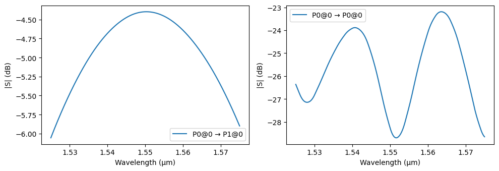
Let’s plot the grating coupler’s S parameters in a denser and wider wavelength grid:
[21]:
wavelengths_dense = np.linspace(1.525, 1.575, 1001)

_ = pf.plot_s_matrix(
    grating_coupler.s_matrix(pf.C_0 / wavelengths_dense), y="dB", input_ports=["P0"]
)
Progress: 100%
Now we can add the gratings to our cascaded filter and, if we so desire, export a layout file for fabrication:
[22]:
netlist_layout = {
    "name": "main",
    "instances": {
        "filter": cascaded_rings,
        "grating0": grating_coupler,
        "grating1": grating_coupler,
        "spacer0": spacer,
        "spacer1": spacer,
    },
    "connections": [
        (("spacer0", "P0"), ("grating0", "P0")),
        (("filter", "P0"), ("spacer0", "P1")),
        (("spacer1", "P0"), ("filter", "P1")),
        (("grating1", "P0"), ("spacer1", "P1")),
    ],
    "ports": [
        ("grating0", "P1"),
        ("grating1", "P1"),
        ("filter", "AD0"),
        ("filter", "AD1"),
        ("filter", "AD2"),
    ],
    "models": [pf.CircuitModel()],
}

layout = pf.component_from_netlist(netlist_layout)

layout.write_gds("cascaded_rings.gds")
[22]:

Once again, we can simulate our full device, but now with a denser and wider wavelength grid to verify the full transmission spectrum between grating couplers. Note that this simulation may take a little longer because we are calculating modes using a fine frequency sweep.
[23]:
wavelengths_wide = np.linspace(1.525, 1.575, 501)
s_layout = layout.s_matrix(frequencies=pf.C_0 / wavelengths_wide)
Starting…
22:36:07 -03 Loading simulation from local cache. View cached task using web UI
             at
             'https://tidy3d.simulation.cloud/workbench?taskId=mo-3f9e77e1-f1b4-
             47bd-bad4-bbfa65df6c89'.
             Loading simulation from local cache. View cached task using web UI
             at
             'https://tidy3d.simulation.cloud/workbench?taskId=mo-0d0d8250-2daa-
             4f88-9f1e-5939c0fb87a7'.
             Loading simulation from local cache. View cached task using web UI
             at
             'https://tidy3d.simulation.cloud/workbench?taskId=fdve-091b68a3-622
             5-4b09-9c8e-da66be0c962e'.
22:36:08 -03 Loading simulation from local cache. View cached task using web UI
             at
             'https://tidy3d.simulation.cloud/workbench?taskId=fdve-5f5063eb-912
             8-4a9d-8ed6-dccf8a21b048'.
             Loading simulation from local cache. View cached task using web UI
             at
             'https://tidy3d.simulation.cloud/workbench?taskId=mo-a7783bbb-7739-
             4e00-9132-4767ad08bd8a'.
             Loading simulation from local cache. View cached task using web UI
             at
             'https://tidy3d.simulation.cloud/workbench?taskId=mo-892161bd-c503-
             46fa-860a-7a117a6fcf5c'.
22:36:09 -03 Loading simulation from local cache. View cached task using web UI
             at
             'https://tidy3d.simulation.cloud/workbench?taskId=fdve-f28dc031-d35
             8-42a2-a6f3-09b557679feb'.
             Loading simulation from local cache. View cached task using web UI
             at
             'https://tidy3d.simulation.cloud/workbench?taskId=fdve-52d99829-57b
             3-485c-9abc-b8697bb5eaaa'.
22:36:10 -03 Loading simulation from local cache. View cached task using web UI
             at
             'https://tidy3d.simulation.cloud/workbench?taskId=fdve-8072ba9f-a59
             d-405d-b45b-06225e052d34'.
22:36:11 -03 Loading simulation from local cache. View cached task using web UI
             at
             'https://tidy3d.simulation.cloud/workbench?taskId=fdve-f17f4b35-5ee
             d-48b9-b0b5-c0b207557312'.
             Loading simulation from local cache. View cached task using web UI
             at
             'https://tidy3d.simulation.cloud/workbench?taskId=fdve-3a3e5f13-371
             5-430d-b7cb-9627c4072f66'.
             Loading simulation from local cache. View cached task using web UI
             at
             'https://tidy3d.simulation.cloud/workbench?taskId=fdve-e381fd74-b97
             b-4fad-aa17-8a05cb318853'.
             Loading simulation from local cache. View cached task using web UI
             at
             'https://tidy3d.simulation.cloud/workbench?taskId=mo-2f753b71-220a-
             40e1-87ef-2d6b5eba90b3'.
             Loading simulation from local cache. View cached task using web UI
             at
             'https://tidy3d.simulation.cloud/workbench?taskId=mo-b3b94e22-b622-
             4bac-871a-fb7079b1f9b2'.
             Loading simulation from local cache. View cached task using web UI
             at
             'https://tidy3d.simulation.cloud/workbench?taskId=mo-250da07e-f01f-
             4ed3-a087-bdc18ee62599'.
             Loading simulation from local cache. View cached task using web UI
             at
             'https://tidy3d.simulation.cloud/workbench?taskId=mo-0a14e030-1f00-
             44cd-a639-6f0a7b7f621b'.
22:36:12 -03 Loading simulation from local cache. View cached task using web UI
             at
             'https://tidy3d.simulation.cloud/workbench?taskId=mo-3c68aa76-d4bb-
             47f0-a077-ee4bbc1da2d2'.
             WARNING: Structure at 'structures[2]' has bounds that extend
             exactly to simulation edges. This can cause unexpected behavior. If
             intending to extend the structure to infinity along one dimension,
             use td.inf as a size variable instead to make this explicit.
             Loading simulation from local cache. View cached task using web UI
             at
             'https://tidy3d.simulation.cloud/workbench?taskId=fdve-ef80768a-c85
             9-4ddb-bc39-f000e3b92c13'.
             WARNING: Structure at 'structures[2]' has bounds that extend
             exactly to simulation edges. This can cause unexpected behavior. If
             intending to extend the structure to infinity along one dimension,
             use td.inf as a size variable instead to make this explicit.
             WARNING: Warning messages were found in the solver log. For more
             information, check 'SimulationData.log' or use
             'web.download_log(task_id)'.
Progress: 100%
[24]:
_, ax = plt.subplots(1, 1, figsize=(9, 3))
ax.plot(wavelengths_wide, 20 * np.log10(np.abs(s_layout["P0@0", "P1@0"])))
_ = ax.set(xlabel="Wavelength (μm)", ylabel="Transmission (dB)", ylim=(-30, None))
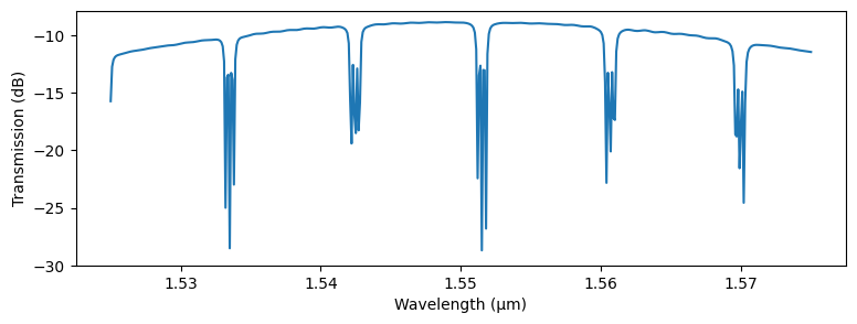
We see that overall filter response has a spectral dependence due to the wavelength response of the grating.
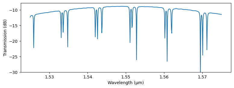
Testing Variations
The Circuit model allows us to test the effect of parameter changes in technologies, components, and models in specific references through the updates keyword argument available in the Circuit model’s start method.
In this case we want to see the effect of changing the resonance frequency of each ring in the filter circuit by modifying the added lengths in each of them. For that, we set a dictionary of updates that first matches each add/drop filter by name ("create_add_drop_…") at any depth of the dependency tree (the value None in the reference specification tuple indicates that whatever follows ca match at any depth). Within each add/drop filter, we select references whose component name starts
with “straight” using a regular expression (.* will match any suffix), and, finally, update the model of those components (which are Waveguide models) with a new length parameter.
[25]:
updates = {
    (None, "create_add_drop_added_length_0_005", "straight.*"): {"model_updates": {"length": 0.0}},
    (None, "create_add_drop_added_length_0_015", "straight.*"): {"model_updates": {"length": 0.02}},
    (None, "create_add_drop_added_length_0_025", "straight.*"): {"model_updates": {"length": 0.06}},
}
updated_s_matrix = layout.s_matrix(
    pf.C_0 / wavelengths_wide, model_kwargs={"updates": updates}
)

_, ax = plt.subplots(1, 1, figsize=(9, 3))
ax.plot(wavelengths_wide, 20 * np.log10(np.abs(updated_s_matrix["P0@0", "P1@0"])))
_ = ax.set(xlabel="Wavelength (μm)", ylabel="Transmission (dB)", ylim=(-30, None))
Starting…
22:36:18 -03 WARNING: Structure at 'structures[2]' has bounds that extend
             exactly to simulation edges. This can cause unexpected behavior. If
             intending to extend the structure to infinity along one dimension,
             use td.inf as a size variable instead to make this explicit.
Progress: 100%
Because we created each add/drop filter as a parametric component with the added_length parameter, we could also obtain the same result by updating the component themselves:
[26]:
updates = {
    (None, "create_add_drop_added_length_0_005"): {"component_updates": {"added_length": 0.0}},
    (None, "create_add_drop_added_length_0_015"): {"component_updates": {"added_length": 0.02}},
    (None, "create_add_drop_added_length_0_025"): {"component_updates": {"added_length": 0.06}},
}
updated_s_matrix = layout.s_matrix(
    pf.C_0 / wavelengths_wide, model_kwargs={"updates": updates}
)

_, ax = plt.subplots(1, 1, figsize=(9, 3))
ax.plot(wavelengths_wide, 20 * np.log10(np.abs(updated_s_matrix["P0@0", "P1@0"])))
_ = ax.set(xlabel="Wavelength (μm)", ylabel="Transmission (dB)", ylim=(-30, None))
Starting…
22:36:22 -03 WARNING: Structure at 'structures[2]' has bounds that extend
             exactly to simulation edges. This can cause unexpected behavior. If
             intending to extend the structure to infinity along one dimension,
             use td.inf as a size variable instead to make this explicit.
Progress: 100%
