Fabrication-Aware Simulation: Two Coupled Ring Resonator Filter

In this notebook we demonstrate how we can perform fabrication-aware simulations in PhotonForge by modeling a 2-ring coupled resonator filter and running a Monte Carlo analysis on key process-variation parameters. We focus on variations in the coupler gap, silicon wafer thickness, and sidewall angle, then visualize their impact on spectral response.
We use the couple mode theory presented in [1] for the filter design.
References
Little, Brent E., et al. “Microring resonator channel dropping filters.” Journal of lightwave technology 1997 15 (6), 998-1005, doi: 10.1109/50.588673.
[1]:
import matplotlib.pyplot as plt
import numpy as np
import pandas as pd
import photonforge as pf
import tidy3d as td
from scipy.signal import find_peaks

# Reduce non-critical Tidy3D logs to keep the notebook output clean
td.config.logging.level = "ERROR"
Setting Up Technology and Simulation Defaults
[2]:
# Load the basic technology
tech = pf.basic_technology()

# Set this as the default technology for all subsequent components
pf.config.default_technology = tech

# Extract the standard single-mode strip waveguide port specification
port_spec = tech.ports["Strip"]

# Set some default parameters for all components (e.g., bend radius)
pf.config.default_kwargs = {
    "radius": 5,  # bend radius in microns
    "port_spec": port_spec,
}

# Define the default mesh refinement level
pf.config.default_mesh_refinement = 15

# Define the wavelength range for optical simulations [µm]
wavelengths = np.linspace(1.543, 1.557, 401)
Parametric 2-Ring Filter Construction
We define a parametric function to build a two coupled ring resonator (2-RR) filter using PhotonForge primitives. The function instantiates two types of couplers — a bus-to-ring coupler and a ring-to-ring coupler — and then stitches them with a netlist that sets up instances, interconnects ports, and exposes the device I/O.
What we parameterize
coupling_length: the straight interaction length in the couplers, controlling the coupling coefficient.
bus_coupling_distance: the nominal gap between the bus waveguide and each ring.
ring_coupling_distance: the nominal gap between the two rings in the inter-ring coupler.
Netlist assembly We instantiate:
Two bus couplers (
bus_coupler0,bus_coupler1)One ring-to-ring coupler (
ring_coupler0)
We then connect their ports to form the 2-RR filter topology and publish four external ports.
Finally, we build the component from the netlist and create a default instance for quick visualization.
Flat-Top (Maximally-Flat) Design Condition
To achieve a flat-top (maximally-flat) passband in the two-ring add–drop filter (with identical rings), we choose the coupling gaps such that the bus-to-ring and ring-to-ring coupling coefficients satisfy the synthesis relation derived in [1]:
\(\kappa_{\text{int}} = \frac{1}{2} \kappa_{\text{ext}}^2\)
where:
\(\kappa_{\text{ext}}\) — bus-to-ring (external) power coupling coefficient (\(\kappa_{\text{ext}} \approx 0.4\) in our design)
\(\kappa_{\text{int}}\) — ring-to-ring (internal) power coupling coefficient (\(\kappa_{\text{int}} \approx 0.08\) in our design)
This condition ensures a maximally-flat spectral response by properly balancing external and internal coupling strengths.
[3]:
@pf.parametric_component
def create_two_rr_filter(
    *,
    coupling_length: float = 13.5,
    bus_coupling_distance: float = 0.7,
    ring_coupling_distance: float = 0.81,
) -> pf.Component:
    """
    Build a 2-ring (2RR) filter from parametric couplers and return the component.
    """
    # Parametric subcomponents
    bus_to_ring = pf.parametric.dual_ring_coupler(
        coupling_distance=bus_coupling_distance,
        coupling_length=coupling_length,
        model=pf.Tidy3DModel(
            verbose=False,
            port_symmetries=[
                ("P1", "P0", "P3", "P2"),
                ("P2", "P3", "P0", "P1"),
                ("P3", "P2", "P1", "P0"),
            ],
        ),
    )

    ring_to_ring = bus_to_ring.copy().update(coupling_distance=ring_coupling_distance)

    # Netlist for assembling the 2RR resonator
    netlist_2RR = {
        "name": "filter",
        "instances": {
            "bus_coupler0": bus_to_ring,
            "bus_coupler1": bus_to_ring,
            "ring_coupler0": ring_to_ring,
        },
        "connections": [
            (("ring_coupler0", "P0"), ("bus_coupler0", "P1")),
            (("bus_coupler1", "P3"), ("ring_coupler0", "P1")),
        ],
        "ports": [
            ("bus_coupler0", "P0"),
            ("bus_coupler1", "P2"),
            ("bus_coupler0", "P2"),
            ("bus_coupler1", "P0"),
        ],
        "models": [pf.CircuitModel()],
    }

    two_rr = pf.component_from_netlist(netlist_2RR)
    return two_rr


two_rr = create_two_rr_filter()
two_rr
[3]:

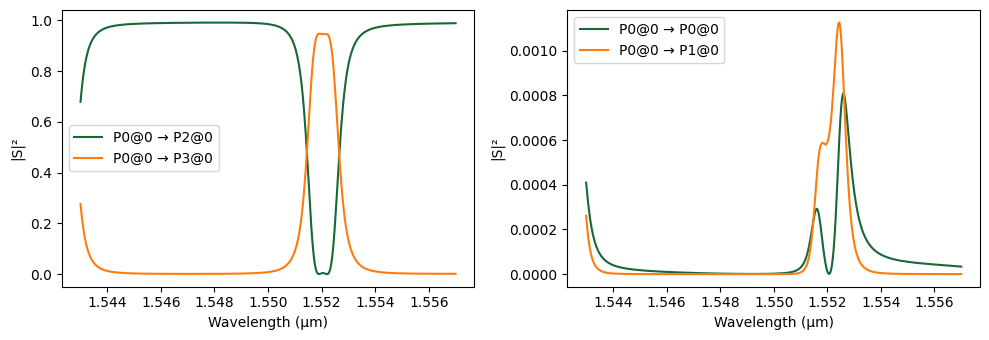
We now compute and visualize the spectral characteristics of the designed 2-RR filter.
[4]:
# Compute the scattering matrix (S-matrix) of the 2RR filter across wavelengths
s_matrix_2rr = two_rr.s_matrix(frequencies=pf.C_0 / wavelengths)

# Plot the S-matrix with input from port P0, showing response in dB
_ = pf.plot_s_matrix(s_matrix_2rr, input_ports=["P0"])
Uploading task 'Mode-Stripwaveguide…'
Uploading task 'Mode-Stripwaveguide…'
Starting task 'Mode-Stripwaveguide': https://tidy3d.simulation.cloud/workbench?taskId=mo-b98f588d-4e81-4d42-a009-5eccf9f8f440
Downloading data from 'Mode-Stripwaveguide'…
Starting task 'Mode-Stripwaveguide': https://tidy3d.simulation.cloud/workbench?taskId=mo-eac5c86d-bb83-4aa5-90e1-712dc93b4bd5
Downloading data from 'Mode-Stripwaveguide'…
Progress: 100%
Monte Carlo Analysis
Parameters under variation
core_thickness (technology): silicon layer thickness, mean 0.22 µm with a 3 nm standard deviation
sidewall_angle (technology): etched sidewall deviation, uniformly sampled between 0° and 5°
bus_coupling_distance (component): coupling gap between bus and ring, mean 0.7 µm with 10 nm σ
ring_coupling_distance (component): gap between rings, mean 0.79 µm with 10 nm σ
[5]:
# Run a Monte Carlo S-matrix analysis to capture fabrication-induced variations
var, results = pf.monte_carlo.s_matrix(
    two_rr,
    pf.C_0 / wavelengths,
    ("core_thickness", "technology", {"value": 0.22, "stdev": 0.003}),
    ("sidewall_angle", "technology", {"value_range": [0, 5]}),
    ("bus_coupling_distance", two_rr, {"value": 0.7, "stdev": 0.01}),
    ("ring_coupling_distance", two_rr, {"value": 0.81, "stdev": 0.01}),
    random_samples=20,  # number of random samples
    corner_samples=2,  # corner cases (extreme combinations)
    random_seed=0,
    show_progress=True,
)
Starting sample 1 of 22…
Uploading task 'Mode-Stripwaveguide…'
Uploading task 'Mode-Stripwaveguide…'
Starting sample 2 of 22…
Uploading task 'Mode-Stripwaveguide…'
Uploading task 'Mode-Stripwaveguide…'
Starting sample 3 of 22…
Uploading task 'Mode-Stripwaveguide…'
Uploading task 'Mode-Stripwaveguide…'
Starting sample 4 of 22…
Uploading task 'Mode-Stripwaveguide…'
Uploading task 'Mode-Stripwaveguide…'
Starting sample 5 of 22…
Uploading task 'Mode-Stripwaveguide…'
Uploading task 'Mode-Stripwaveguide…'
Starting sample 6 of 22…
Uploading task 'Mode-Stripwaveguide…'
Uploading task 'Mode-Stripwaveguide…'
Starting sample 7 of 22…
Uploading task 'Mode-Stripwaveguide…'
Uploading task 'Mode-Stripwaveguide…'
Starting sample 8 of 22…
Uploading task 'Mode-Stripwaveguide…'
Uploading task 'Mode-Stripwaveguide…'
Starting sample 9 of 22…
Uploading task 'Mode-Stripwaveguide…'
Uploading task 'Mode-Stripwaveguide…'
Starting sample 10 of 22…
Uploading task 'Mode-Stripwaveguide…'
Uploading task 'Mode-Stripwaveguide…'
Starting sample 11 of 22…
Starting task 'Mode-Stripwaveguide': https://tidy3d.simulation.cloud/workbench?taskId=mo-8f7da2e2-6546-4f4d-99c9-3f9a0eae6ec5
Uploading task 'Mode-Stripwaveguide…'
Uploading task 'Mode-Stripwaveguide…'
Starting sample 12 of 22…
Starting task 'Mode-Stripwaveguide': https://tidy3d.simulation.cloud/workbench?taskId=mo-a61887e3-eb8e-4de4-b4ca-604e056c705e
Downloading data from 'Mode-Stripwaveguide'…
Uploading task 'Mode-Stripwaveguide…'
Uploading task 'Mode-Stripwaveguide…'
Starting sample 13 of 22…
Starting task 'Mode-Stripwaveguide': https://tidy3d.simulation.cloud/workbench?taskId=mo-76aeae53-2690-4698-a158-2ae8ad3bb7c3
Starting task 'Mode-Stripwaveguide': https://tidy3d.simulation.cloud/workbench?taskId=mo-b2fc6d6b-8eae-4359-8c01-2753a2d2f6ac
Starting task 'Mode-Stripwaveguide': https://tidy3d.simulation.cloud/workbench?taskId=mo-6ea6c574-88c5-4ca5-883a-c40f7f91e3e5
Uploading task 'Mode-Stripwaveguide…'
Uploading task 'Mode-Stripwaveguide…'
Downloading data from 'Mode-Stripwaveguide'…
Starting task 'Mode-Stripwaveguide': https://tidy3d.simulation.cloud/workbench?taskId=mo-926f0ef8-1916-467b-a02d-7ee44b8f8a36
Downloading data from 'Mode-Stripwaveguide'…
Starting sample 14 of 22…
Starting task 'Mode-Stripwaveguide': https://tidy3d.simulation.cloud/workbench?taskId=mo-fa2ce6a5-74fe-4dbe-9f78-2c0d0b351d2e
Downloading data from 'Mode-Stripwaveguide'…
Downloading data from 'Mode-Stripwaveguide'…
Uploading task 'Mode-Stripwaveguide…'
Uploading task 'Mode-Stripwaveguide…'
Starting task 'Mode-Stripwaveguide': https://tidy3d.simulation.cloud/workbench?taskId=mo-a9977406-6c21-4fd8-8831-5d543b1701e7
Downloading data from 'Mode-Stripwaveguide'…
Starting sample 15 of 22…
Downloading data from 'Mode-Stripwaveguide'…
Uploading task 'Mode-Stripwaveguide…'
Downloading data from 'Mode-Stripwaveguide'…
Uploading task 'Mode-Stripwaveguide…'
Starting task 'Mode-Stripwaveguide': https://tidy3d.simulation.cloud/workbench?taskId=mo-11d73b1c-e1a5-4f48-99d1-333ed7d29ee8
Downloading data from 'Mode-Stripwaveguide'…
Starting sample 16 of 22…
Starting task 'Mode-Stripwaveguide': https://tidy3d.simulation.cloud/workbench?taskId=mo-963f5b01-ec99-4360-9371-8929ebfee8ba
Starting task 'Mode-Stripwaveguide': https://tidy3d.simulation.cloud/workbench?taskId=mo-ded3a1a9-f76a-4382-9f18-a833d09e867f
Uploading task 'Mode-Stripwaveguide…'
Uploading task 'Mode-Stripwaveguide…'
Downloading data from 'Mode-Stripwaveguide'…
Downloading data from 'Mode-Stripwaveguide'…
Starting task 'Mode-Stripwaveguide': https://tidy3d.simulation.cloud/workbench?taskId=mo-fdbb12ff-6b68-4b55-94e5-8f96b06c155a
Starting sample 17 of 22…
Downloading data from 'Mode-Stripwaveguide'…
Starting task 'Mode-Stripwaveguide': https://tidy3d.simulation.cloud/workbench?taskId=mo-587c0a85-f269-415f-82c1-bddf6b3077be
Starting task 'Mode-Stripwaveguide': https://tidy3d.simulation.cloud/workbench?taskId=mo-6dff947d-3e8e-49cc-8b0c-c544a6867bab
Starting task 'Mode-Stripwaveguide': https://tidy3d.simulation.cloud/workbench?taskId=mo-70259dc6-f927-451d-8f43-c89090d65a20
Starting task 'Mode-Stripwaveguide': https://tidy3d.simulation.cloud/workbench?taskId=mo-a77c9c18-aff7-4452-a932-ddaf0707730a
Downloading data from 'Mode-Stripwaveguide'…
Downloading data from 'Mode-Stripwaveguide'…
Uploading task 'Mode-Stripwaveguide…'
Uploading task 'Mode-Stripwaveguide…'
Downloading data from 'Mode-Stripwaveguide'…
Downloading data from 'Mode-Stripwaveguide'…
Starting sample 18 of 22…
Uploading task 'Mode-Stripwaveguide…'
Starting task 'Mode-Stripwaveguide': https://tidy3d.simulation.cloud/workbench?taskId=mo-8e7ccaba-c734-4ad3-a7b6-60cf813e54d4
Uploading task 'Mode-Stripwaveguide…'
Starting sample 19 of 22…
Uploading task 'Mode-Stripwaveguide…'
Downloading data from 'Mode-Stripwaveguide'…
Uploading task 'Mode-Stripwaveguide…'
Starting task 'Mode-Stripwaveguide': https://tidy3d.simulation.cloud/workbench?taskId=mo-d35783f3-d459-4e9a-94d7-0ffb0e843810
Starting task 'Mode-Stripwaveguide': https://tidy3d.simulation.cloud/workbench?taskId=mo-bdd8ea3f-ffa5-4636-8581-14d21bb9bcc8
Starting task 'Mode-Stripwaveguide': https://tidy3d.simulation.cloud/workbench?taskId=mo-5197c689-dbd5-4920-8702-e58ff5cb09c3
Starting task 'Mode-Stripwaveguide': https://tidy3d.simulation.cloud/workbench?taskId=mo-9b43ce58-b895-44a3-90d3-8136ff478db4
Starting sample 20 of 22…
Uploading task 'Mode-Stripwaveguide…'
Uploading task 'Mode-Stripwaveguide…'
Downloading data from 'Mode-Stripwaveguide'…
Downloading data from 'Mode-Stripwaveguide'…
Starting sample 21 of 22…
Downloading data from 'Mode-Stripwaveguide'…
Downloading data from 'Mode-Stripwaveguide'…
Starting task 'Mode-Stripwaveguide': https://tidy3d.simulation.cloud/workbench?taskId=mo-72235a6d-533f-4b47-baea-a014f3a7b625
Uploading task 'Mode-Stripwaveguide…'
Uploading task 'Mode-Stripwaveguide…'
Starting task 'Mode-Stripwaveguide': https://tidy3d.simulation.cloud/workbench?taskId=mo-6553664e-2322-4e4d-bc48-f643ee9f0137
Starting task 'Mode-Stripwaveguide': https://tidy3d.simulation.cloud/workbench?taskId=mo-a3025469-e011-48ee-af3a-343a566b61a1
Starting sample 22 of 22…
Uploading task 'Mode-Stripwaveguide…'
Downloading data from 'Mode-Stripwaveguide'…
Uploading task 'Mode-Stripwaveguide…'
Starting task 'Mode-Stripwaveguide': https://tidy3d.simulation.cloud/workbench?taskId=mo-38f908bb-3a57-427e-a177-60d72a53e790
Starting task 'Mode-Stripwaveguide': https://tidy3d.simulation.cloud/workbench?taskId=mo-29552dd1-55fa-4821-9da1-11d01f77a42e
Sample 1 done.
Sample 2 done.
Sample 3 done.
Sample 4 done.
Sample 5 done.
Sample 6 done.
Sample 7 done.
Sample 8 done.
Sample 9 done.
Downloading data from 'Mode-Stripwaveguide'…
Downloading data from 'Mode-Stripwaveguide'…
Downloading data from 'Mode-Stripwaveguide'…
Sample 10 done.
Downloading data from 'Mode-Stripwaveguide'…
Starting task 'Mode-Stripwaveguide': https://tidy3d.simulation.cloud/workbench?taskId=mo-e98c91a2-ef04-40f7-a39e-0866b5b57158
Starting task 'Mode-Stripwaveguide': https://tidy3d.simulation.cloud/workbench?taskId=mo-39164912-7760-42fc-9500-3b842f947e58
Downloading data from 'Mode-Stripwaveguide'…
Downloading data from 'Mode-Stripwaveguide'…
Starting task 'Mode-Stripwaveguide': https://tidy3d.simulation.cloud/workbench?taskId=mo-29fef227-0032-49f2-b021-b3ef4f02c10f
Sample 11 done.
Sample 12 done.
Downloading data from 'Mode-Stripwaveguide'…
Starting task 'Mode-Stripwaveguide': https://tidy3d.simulation.cloud/workbench?taskId=mo-4e3df322-a776-4b02-af5a-264f3fffb65b
Sample 13 done.
Starting task 'Mode-Stripwaveguide': https://tidy3d.simulation.cloud/workbench?taskId=mo-f26c7c7d-05f6-4c4d-8a01-f3b36e6f5614
Downloading data from 'Mode-Stripwaveguide'…
Sample 14 done.
Downloading data from 'Mode-Stripwaveguide'…
Starting task 'Mode-Stripwaveguide': https://tidy3d.simulation.cloud/workbench?taskId=mo-2fecf9ce-a77b-41ca-aea7-e6150a2a3f00
Sample 15 done.
Downloading data from 'Mode-Stripwaveguide'…
Starting task 'Mode-Stripwaveguide': https://tidy3d.simulation.cloud/workbench?taskId=mo-acbfc8b7-d45e-4680-ac43-75f6162b5158
Starting task 'Mode-Stripwaveguide': https://tidy3d.simulation.cloud/workbench?taskId=mo-27397bc3-807e-4696-ba83-342f40c3781c
Sample 16 done.
Downloading data from 'Mode-Stripwaveguide'…
Starting task 'Mode-Stripwaveguide': https://tidy3d.simulation.cloud/workbench?taskId=mo-ddeadd5c-8deb-47a7-a9b2-7961c3f4a848
Starting task 'Mode-Stripwaveguide': https://tidy3d.simulation.cloud/workbench?taskId=mo-7c2e6436-f88c-4ac2-9a11-8882ae754c43
Downloading data from 'Mode-Stripwaveguide'…
Downloading data from 'Mode-Stripwaveguide'…
Downloading data from 'Mode-Stripwaveguide'…
Starting task 'Mode-Stripwaveguide': https://tidy3d.simulation.cloud/workbench?taskId=mo-8acfceb9-6199-4abb-9c63-f9a8dd148c40
Starting task 'Mode-Stripwaveguide': https://tidy3d.simulation.cloud/workbench?taskId=mo-273e1cba-7052-458c-91ef-d7bda58f8ac9
Starting task 'Mode-Stripwaveguide': https://tidy3d.simulation.cloud/workbench?taskId=mo-1a1d310f-0d7b-45cb-b6ec-de4d9fa57d5b
Downloading data from 'Mode-Stripwaveguide'…
Downloading data from 'Mode-Stripwaveguide'…
Downloading data from 'Mode-Stripwaveguide'…
Sample 17 done.
Starting task 'Mode-Stripwaveguide': https://tidy3d.simulation.cloud/workbench?taskId=mo-1d3ff6e6-83c0-4a84-a4ef-f06299947ed0
Sample 18 done.
Downloading data from 'Mode-Stripwaveguide'…
Starting task 'Mode-Stripwaveguide': https://tidy3d.simulation.cloud/workbench?taskId=mo-951fa1f3-6f45-4ed0-86ba-b1866c948483
Starting task 'Mode-Stripwaveguide': https://tidy3d.simulation.cloud/workbench?taskId=mo-00159e4f-eb68-4ad4-9ed0-537d0a483c22
Sample 19 done.
Starting task 'Mode-Stripwaveguide': https://tidy3d.simulation.cloud/workbench?taskId=mo-2977430b-efbc-4e17-906a-3c815227d6dc
Starting task 'Mode-Stripwaveguide': https://tidy3d.simulation.cloud/workbench?taskId=mo-82544350-0224-41ba-8703-0768264463f0
Downloading data from 'Mode-Stripwaveguide'…
Downloading data from 'Mode-Stripwaveguide'…
Sample 20 done.
Downloading data from 'Mode-Stripwaveguide'…
Downloading data from 'Mode-Stripwaveguide'…
Sample 21 done.
Sample 22 done.
All samples done!
[6]:
fig, ax = plt.subplots(1, 1)

for *_, s_matrix in results:
    ax.plot(
        s_matrix.wavelengths,
        20 * np.log10(np.abs(s_matrix[("P0@0", "P3@0")])),
        alpha=0.5,
        color="tab:orange",
    )

_ = ax.set(ylim=(-20, 0), xlabel="λ (µm)", ylabel="Transmission (dB)")
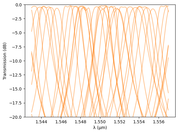
Discussion of Fabrication-Aware Results
The Monte Carlo simulation shows that fabrication variations can significantly impact the spectral response of the 2-RR filter:
- Resonance wavelength drift:The resonance positions vary substantially between samples, indicating that small deviations in silicon thickness, sidewall angle, or coupling gaps lead to noticeable phase shifts and effective index changes.This explains why thermal tuning (via integrated heaters) is almost always required in fabricated ring filters to fine-tune or align the resonance wavelengths post-fabrication.
- Insertion loss variation:The simulated through-port transmission fluctuates between approximately 0.3 dB and 1.0 dB, demonstrating that while loss performance changes slightly, the filter remains fairly robust to process deviations in this respect.
Overall, the analysis illustrates how PhotonForge’s fabrication-aware modeling can predict both resonance misalignment and performance spread, allowing designers to anticipate tuning requirements and optimize yield.
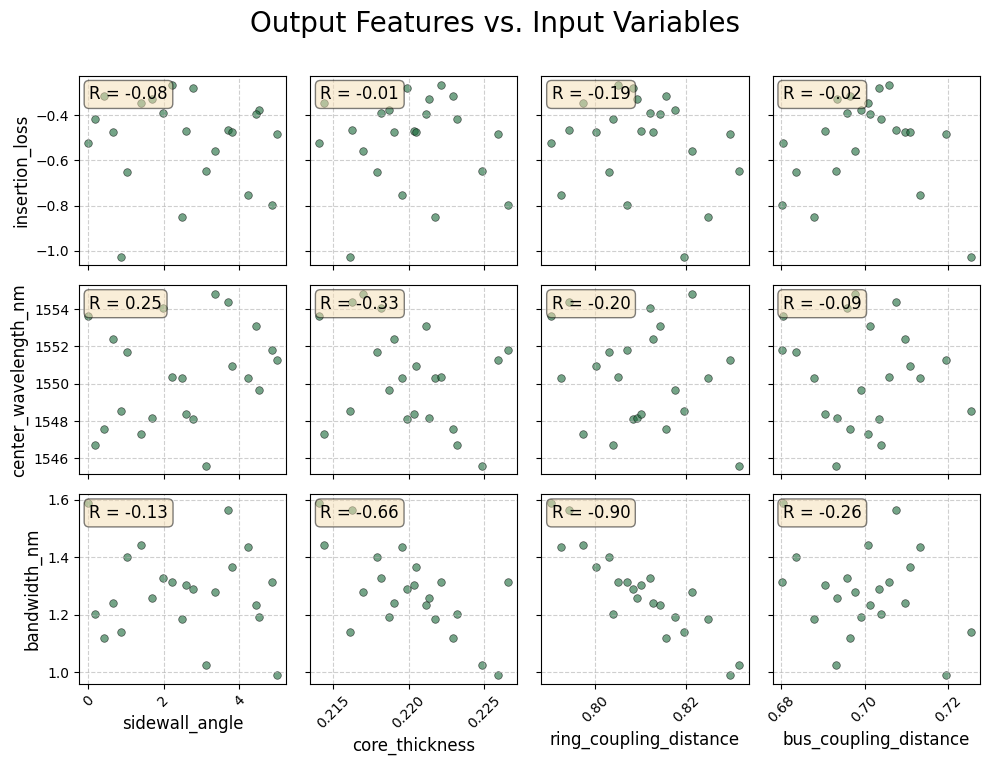
Correlation Analysis
Monte Carlo analysis allows for the extraction of correlations between a device’s response and its input variables. This section demonstrates the correlation analysis process. Critically, accurate results with four input variables require hundreds of data points. The findings presented here are, therefore, purely illustrative and not statistically significant.
Feature extraction
In this section we extract three filter features from each simulated S-matrix so we can study their correlation with fabrication variables. We target the resonance closest to a reference wavelength \(\lambda_0\) (default \(1.55 \mu\)m) and compute:
Center wavelength \(\lambda_c\): the midpoint between the two 3-dB crossing wavelengths around the chosen resonance.
Insertion loss IL (in dB): transmission value at the center wavelength.
3-dB bandwidth \(\Delta\lambda_{3,\text{dB}}\): difference between the right and left 3-dB crossing wavelengths.
[7]:
def extract_filter_features(s_matrix, target_wavelength=1.55):
    """
    Extracts key features (insertion loss, center wavelength, bandwidth)
    from an optical filter's S-matrix data.

    This function identifies the resonance dip closest to a target wavelength
    and calculates its characteristics.

    Args:
        s_matrix: The S-matrix object from the simulation.
        target_wavelength (float): The wavelength (in µm) around which to
                                   search for the primary resonance.
                                   Defaults to 1.55 µm.

    Returns:
        dict: A dictionary containing the calculated 'center_wavelength',
              'insertion_loss' (in dB), and 'bandwidth' (in µm).
              Returns None if no resonance is found.
    """
    wavelengths = s_matrix.wavelengths
    # Calculate transmission in dB
    transmission_db = 20 * np.log10(np.abs(s_matrix[("P0@0", "P3@0")]))

    # The 'prominence' parameter helps ignore minor ripples and noise.
    peak_indices, _ = find_peaks(transmission_db, prominence=1)

    if peak_indices.size == 0:
        print("Warning: No resonance peaks found.")
        return None

    # Find the peak/resonance closest to the target wavelength
    resonant_wavelengths = wavelengths[peak_indices]
    closest_peak_index = peak_indices[
        np.argmin(np.abs(resonant_wavelengths - target_wavelength))
    ]

    # --- 1. Calculate Maximum Transmission Wavelength and Insertion Loss ---
    max_wavelength = wavelengths[closest_peak_index]
    insertion_loss = transmission_db[closest_peak_index]

    # --- 2. Calculate 3-dB Bandwidth ---
    # The 3-dB level is 3 dB below the maximum transmission value (the IL)
    three_db_level = insertion_loss - 3

    # Find where the transmission crosses the 3-dB level on both sides of the resonance
    # Split the transmission data at the resonance point
    left_side = transmission_db[:closest_peak_index]
    right_side = transmission_db[closest_peak_index:]

    # Find the indices where the transmission is greater than the 3-dB level
    left_indices_below_3db = np.where(left_side < three_db_level)[0]
    right_indices_below_3db = np.where(right_side < three_db_level)[0]

    if left_indices_below_3db.size == 0 or right_indices_below_3db.size == 0:
        bandwidth = np.nan  # Use NaN for cases where bandwidth can't be found
    else:
        # Get the points just before and after the crossing
        left_cross_idx = left_indices_below_3db[-1]
        right_cross_idx = right_indices_below_3db[0] + closest_peak_index

        # Interpolate to find the exact wavelength at the 3dB crossing for better accuracy
        w_left = np.interp(
            three_db_level,
            [transmission_db[left_cross_idx], transmission_db[left_cross_idx + 1]],
            [wavelengths[left_cross_idx], wavelengths[left_cross_idx + 1]],
        )

        w_right = np.interp(
            three_db_level,
            [transmission_db[right_cross_idx - 1], transmission_db[right_cross_idx]],
            [wavelengths[right_cross_idx - 1], wavelengths[right_cross_idx]],
        )

        # Compute bandwidth and center wavelength from crossings
        bandwidth = w_right - w_left
        center_wavelength = (w_right + w_left) / 2
        insertion_loss = transmission_db[(left_cross_idx + right_cross_idx) // 2]

    return {
        "center_wavelength": center_wavelength,
        "insertion_loss": insertion_loss,
        "bandwidth": bandwidth,
    }
Correlation Matrix
Interpretation
R ≈ +1: Strong positive correlation — as the fabrication parameter increases, the feature value increases.
R ≈ -1: Strong negative correlation — the feature decreases as the parameter increases.
R ≈ 0: Weak or no linear correlation.
This visualization allows us to directly identify which fabrication tolerances most strongly impact spectral behavior such as resonance shift, insertion loss, or bandwidth broadening.
Important note: The correlation results shown here are intended for demonstration only and are not statistically valid because of small number of data points.
[8]:
def run_correlation_analysis(variables, simulation_results, target_wavelength=1.55):
    """
    Processes Monte Carlo simulation results to visualize the relationship
    and correlation between each input variable and each output filter feature.

    Args:
        variables (list): The list of RandomVariable objects from the simulation.
        simulation_results (list): The list of result tuples from the simulation.
                                     Each tuple contains the input values and the s_matrix.
        target_wavelength (float): The target wavelength in micrometers.
    """
    data = []
    variable_names = [v.name for v in variables]

    print("Processing simulation results...")
    for result in simulation_results:
        s_matrix = result[-1]
        input_values = result[:-1]
        features = extract_filter_features(
            s_matrix, target_wavelength=target_wavelength
        )

        if features:
            run_data = {name: val for name, val in zip(variable_names, input_values)}
            run_data.update(features)
            data.append(run_data)

    if not data:
        print("Could not extract features from any simulation run. Aborting.")
        return

    print(f"Successfully processed {len(data)} data points.")
    df = pd.DataFrame(data)
    df["center_wavelength"] *= 1e3
    df["bandwidth"] *= 1e3
    df = df.rename(
        columns={
            "center_wavelength": "center_wavelength_nm",
            "bandwidth": "bandwidth_nm",
        }
    )

    print("\n--- Data Head ---")
    print(df.head())

    output_feature_names = ["insertion_loss", "center_wavelength_nm", "bandwidth_nm"]

    print("\n--- Generating Custom Scatter Plot Grid with Correlation Values ---")

    n_outputs = len(output_feature_names)
    n_inputs = len(variable_names)

    fig, axes = plt.subplots(
        n_outputs, n_inputs, figsize=(10, 8), sharex="col", sharey="row"
    )

    if n_outputs == 1 or n_inputs == 1:
        axes = np.array(axes).reshape(n_outputs, n_inputs)

    for i, out_feature in enumerate(output_feature_names):
        for j, in_variable in enumerate(variable_names):
            ax = axes[i, j]
            ax.scatter(
                df[in_variable],
                df[out_feature],
                alpha=0.6,
                s=30,
                edgecolor="k",
                linewidth=0.5,
            )
            corr = df[in_variable].corr(df[out_feature])
            corr_text = f"R = {corr:.2f}"
            ax.text(
                0.05,
                0.95,
                corr_text,
                transform=ax.transAxes,
                fontsize=12,
                verticalalignment="top",
                bbox=dict(boxstyle="round,pad=0.3", facecolor="wheat", alpha=0.5),
            )
            if j == 0:
                ax.set_ylabel(out_feature, fontsize=12)
            if i == n_outputs - 1:
                ax.set_xlabel(in_variable, fontsize=12)

            ax.tick_params(axis="x", rotation=45)
            ax.grid(True, linestyle="--", alpha=0.6)

    fig.suptitle("Output Features vs. Input Variables", fontsize=20)
    plt.tight_layout(rect=[0, 0.03, 1, 0.97])
    plt.show()


run_correlation_analysis(var, results)
Processing simulation results...
Successfully processed 22 data points.

--- Data Head ---
   sidewall_angle  core_thickness  ring_coupling_distance  \
0        5.000000        0.225880                0.829600
1        0.000000        0.214120                0.790400
2        4.517759        0.218700                0.817602
3        4.244655        0.219547                0.792679
4        2.785838        0.219909                0.808466

   bus_coupling_distance  center_wavelength_nm  insertion_loss  bandwidth_nm
0               0.719600           1551.269666       -0.437802      0.960668
1               0.680400           1553.621434       -0.432437      1.577132
2               0.699238           1549.720321       -0.360114      1.189358
3               0.713226           1550.306610       -0.744130      1.416780
4               0.703479           1548.111937       -0.212003      1.256126

--- Generating Custom Scatter Plot Grid with Correlation Values ---