Data Model
The data model is used when the S parameters for a component are available as value arrays, for example, loaded from a Touchstone (snp) file. This type of model allows the use of data imported from alternative sources and, in particular, experimental data to be used for simulation.
[1]:
import numpy as np
import photonforge as pf
from matplotlib import pyplot as plt

pf.config.default_technology = pf.basic_technology()
Sample Data Generation
For practical reasons, we’ll first create a Touchstone file with data from a Tidy3D model simulation, instead of running an actual experiment. The following component is not practical, but it is a small example that provides an interesting S parameter curve.
[2]:
component = pf.Component("MAIN")

component.add(
    "WG_CORE",
    pf.Path((0, -2.5), 0.5)
    .segment((0, -2))
    .segment((0, -1.5), 0.2)
    .segment((0, 1.5))
    .segment((0, 2), 0.5)
    .segment((0, 2.5)),
    "SLAB",
    *[pf.Rectangle(center=(0, i * 0.4), size=(2, 0.25)) for i in range(-4, 5)]
)

component.add("WG_CLAD", pf.envelope(component, 1, trim_y_min=True, trim_y_max=True))

component.add_port(component.detect_ports())

component.add_model(pf.Tidy3DModel(port_symmetries=[("P1", "P0")]), "Tidy3D")

component
[2]:

The S matrix values will be computed using 21 equally-spaced points in wavelength domain:
[3]:
s_matrix = component.s_matrix(pf.C_0 / np.linspace(1.3, 1.7, 21))

plt.plot(pf.C_0 / s_matrix.frequencies, np.abs(s_matrix["P0@0", "P0@0"]), label="Reflection")
plt.plot(pf.C_0 / s_matrix.frequencies, np.abs(s_matrix["P0@0", "P1@0"]), label="Transmission")
plt.xlabel("Wavelength (μm)")
_ = plt.legend()
Uploading task 'P0@0…'
Starting task 'P0@0': https://tidy3d.simulation.cloud/workbench?taskId=fdve-301c5f88-d69b-4e5e-b8a9-0cc47c53f37d
Downloading data from 'P0@0'…
Progress: 100%
The data is written to a Touchstone file to be loaded as if it were experimental data.
[4]:
_ = s_matrix.write_snp("data.s2p")
Loading S Matrix Data
Loading Touchstone files can be done with the load_snp function or the SMatrix.load_snp method. The former returns an array with the S matrix values and another with their corresponding frequencies, and the latter creates an S matrix object directly and is usually easier to use.
[5]:
loaded_s_matrix = pf.SMatrix.load_snp("data.s2p")

data_model = pf.DataModel(loaded_s_matrix, interpolation_method="linear")
The data model can be used just as any other model to generate S parameters for the component they are assigned to. The only condition that must be respected is that the number of ports/modes of the component must match the model’s.
For example, we can create a black-box components and use our experimental data model to include the component in larger systems with circuit models.
[6]:
black_box = pf.Component("BB")

black_box.add_port(pf.Port((0, 0), 0, "Strip"), "P0")
black_box.add_port(pf.Port((1, 0), 180, "Rib"), "P1")

black_box.add_model(data_model, "Data")

black_box
[6]:

[7]:
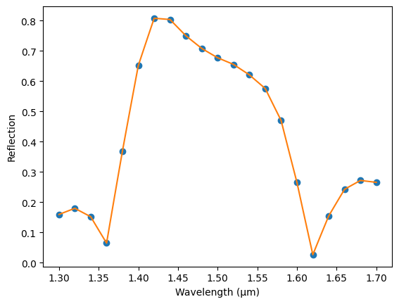
freqs = pf.C_0 / np.linspace(1.3, 1.7, 101)
s_data = black_box.s_matrix(freqs)

plt.plot(pf.C_0 / s_matrix.frequencies, np.abs(s_matrix["P0@0", "P0@0"]), "o")
plt.plot(pf.C_0 / s_data.frequencies, np.abs(s_data["P0@0", "P0@0"]))
plt.xlabel("Wavelength (μm)")
_ = plt.ylabel("Reflection")
Progress: 100%
Interpolation
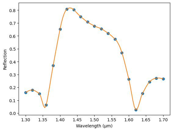
Note that the S matrix retrieved from the data model earlier used a different set of frequency points from the original. The data model computes the S parameters using linear interpolation by default, but that can be easily changed to a few other methods, documented in the data model constructor. Let’s use the "akima" method for a smoother interpolation:
[8]:
model = pf.DataModel(loaded_s_matrix, interpolation_method="akima")

s_data = model.s_matrix(component, freqs)

plt.plot(pf.C_0 / s_matrix.frequencies, np.abs(s_matrix["P0@0", "P0@0"]), "o")
plt.plot(pf.C_0 / s_data.frequencies, np.abs(s_data["P0@0", "P0@0"]))
plt.xlabel("Wavelength (μm)")
_ = plt.ylabel("Reflection")
Progress: 100%
By default, the interpolation is applied to the magnitude and phases independently. It is also possible to interpolate using the real and imaginary components of the S parameters, but that usually leads to large phase jumps.
Data model from an S-matrix array
You can also create a DataModel directly from s_array and frequencies.
In the usual S-parameter convention, s_ij means input at port ``j`` and output at port ``i``. In PhotonForge, the dictionary key order uses (ports[i], ports[j]), and the array-to-dictionary conversion is:
s_dict[(ports[i], ports[j])] = s_array[:, j, i]
So when moving from matrix notation to the PhotonForge dictionary mapping, you should swap i and j in the array indexing. This is especially important for nonreciprocal devices, where forward and reverse transmission are different.
[9]:
# Shape: (F, N, N) with N=2 ports
s_array = np.zeros((len(freqs), 2, 2), dtype=complex)
phi = np.linspace(0, np.pi, len(freqs))
# Add slight frequency-domain amplitude variation
amp_fwd = 0.45 + 0.05 * np.cos(2.5 * phi)
amp_rev = 0.35 + 0.04 * np.sin(2.5 * phi)
# Nonreciprocal transmission terms:
# Typical s_ij: input at j, output at i
# PhotonForge mapping: s_dict[(ports[i], ports[j])] = s_array[:, j, i]
s_array[:, 1, 0] = amp_fwd * np.exp(1j * phi)
s_array[:, 0, 1] = amp_rev * np.exp(-1.2j * phi)
# Small reflections with mild frequency variation
s_array[:, 0, 0] = 0.08 + 0.01 * np.sin(3 * phi)
s_array[:, 1, 1] = (0.12 + 0.015 * np.cos(1.5 * phi)) * np.exp(0.5j * phi)
data_model_from_array = pf.DataModel(
s_array=s_array,
frequencies=freqs,
interpolation_method="linear",
)
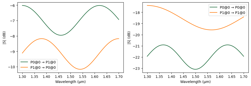
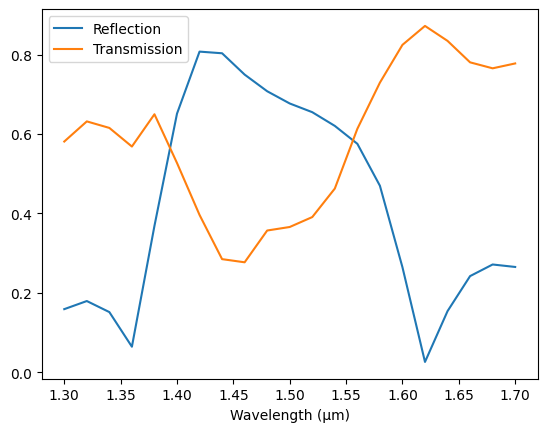
black_box.add_model(data_model_from_array, "Array Data")
s_matrix_array = data_model_from_array.s_matrix(black_box, freqs)
_ = pf.plot_s_matrix(s_matrix_array, y="dB")
Progress: 100%