Importing a GDSII/OASIS Layout

Importing an existing GDSII or OASIS layout file is easy with PhotonForge. Each cell in the layout is loaded as a component and the hierarchical structure in the file is preserved as PhotonForge references.

One important aspect to notice is that GDSII and OASIS files do not include a standard way to specify the PDK they use. That means that we are responsible for loading the appropriate technology for the file we want to import.

In this example, we’ll load the GDSII file created in the Mach-Zehnder interferometer example. That file was created for use with the basic technology included in PhotonForge, but with a strip waveguide profile with 450 nm core, so we first set that as our default technology.

import photonforge as pf

pf.config.default_technology = pf.basic_technology(strip_width=0.45)

With the technology set, loading the layout is done with the load_layout function, which returns a dictionary of components by name.

# Load the gds file
gds_file = "../examples/MZI.gds"
components = pf.load_layout(gds_file)
print("Components:", list(components.keys()))

Components: ['DELAY_STRAIGHT_10', 'BEND', 'DELAY_ARM_0', 'MZI', 'COUPLER', 'DELAY_ARM_10']

components["COUPLER"]

If we don’t know which of the components are at the top-level in the cell hierarchy in the layout, the find_top_level function can provide that information.

top_level = pf.find_top_level(*components.values())
print("Top level components:", [component.name for component in top_level])

Top level components: ['MZI']

We can visualize the dependency tree of any component using the tree_view function (static or interactively):

mzi = components["MZI"]
mzi.tree_view()

MZI
├─ COUPLER
├─ DELAY_ARM_0
│  └─ BEND
└─ DELAY_ARM_10
   ├─ DELAY_STRAIGHT_10
   └─ BEND

mzi.tree_view(interactive=True)

MZI

COUPLER

DELAY_ARM_0

BEND

DELAY_ARM_10

DELAY_STRAIGHT_10

BEND

Because we generated the default technology with the appropriate strip waveguide profile for this layout, adding ports is easy with port auto-detection:

ports = mzi.detect_ports(["Strip"])
print("Detected ports:\n" + "\n".join([f" - {p}" for p in ports]))

Detected ports:
 - Port at (-4.25, -6.55) at 90 deg of type Strip waveguide
 - Port at (-4.25, 0) at 270 deg of type Strip waveguide
 - Port at (18.75, -6.55) at 90 deg of type Strip waveguide
 - Port at (18.75, 0) at 270 deg of type Strip waveguide

mzi.add_port(ports, "P")
mzi

We can continue adding ports and models to all sub-components loaded from the layout to replicate the circuit simulation used in the original example.

However, if the component tree is large, this process can become very tedious. Instead, we can add the ports only to the leaf components in the tree (components without sub-components) and process all others automatically.

We start by finding all leaf components:

leaves = [c.name for c in mzi.dependencies() if len(c.references) == 0]
leaves

['COUPLER', 'BEND', 'DELAY_STRAIGHT_10']

Each of those components we have to process individually, because they have unique characteristics:

coupler = components["COUPLER"]

coupler.add_port(coupler.detect_ports(["Strip"]), "P")
assert len(coupler.ports) == 4

coupler.add_model(
    pf.Tidy3DModel(
        port_symmetries=[
            ("P1", "P0", "P3", "P2"),
            ("P2", "P3", "P0", "P1"),
            ("P3", "P2", "P1", "P0"),
        ],
        verbose=False,
    ),
    "Tidy3DModel",
)
coupler

bend = components["BEND"]

bend.add_port(bend.detect_ports(["Strip"]), "P")
assert len(bend.ports) == 2

bend.add_model(pf.Tidy3DModel(port_symmetries=[("P1", "P0")]), "Tidy3DModel")
bend

straight = components["DELAY_STRAIGHT_10"]

straight.add_port(straight.detect_ports(["Strip"]), "P")
assert len(straight.ports) == 2

straight.add_model(pf.WaveguideModel(verbose=False), "WaveguideModel")
straight

Now, for all intermediate components in the hierarchy and the top level MZI we simply want to add the ports derived from their sub-components and a circuit models to combine their S matrices. The method add_reference_ports was created exactly for this purpose:

mzi.add_reference_ports(add_model=pf.CircuitModel(), include_dependencies=True)

for component in [mzi] + mzi.dependencies():
    print(
        f"{component.name}: ports = {list(component.ports)}; active model = {component.active_model}"
    )

MZI: ports = ['P3', 'P2', 'P1', 'P0']; active model = CircuitModel
COUPLER: ports = ['P3', 'P2', 'P1', 'P0']; active model = Tidy3DModel
DELAY_ARM_0: ports = ['P1', 'P0']; active model = CircuitModel
BEND: ports = ['P1', 'P0']; active model = Tidy3DModel
DELAY_ARM_10: ports = ['P1', 'P0']; active model = CircuitModel
DELAY_STRAIGHT_10: ports = ['P1', 'P0']; active model = WaveguideModel

We may check the netlists of the components with circuit models to make sure we connected all sub-components correctly. If any sub-component is disconnected or missing a model, we’ll get an error or warning when computing the scattering matrix.

import numpy as np

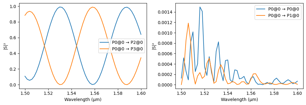
s_matrix = mzi.s_matrix(pf.C_0 / np.linspace(1.5, 1.6, 51))

_ = pf.plot_s_matrix(s_matrix, input_ports=["P0"])

Loading cached simulation from .tidy3d/pf_cache/DP7/ms_info-A5FYNSQPYOICFG7TY2JXZTV6HTGBCIQTJ7ZWD6JE75WKY6CPKDAQ.json.
Loading cached simulation from .tidy3d/pf_cache/GR4/ms_info-PLFVDCS2W7HQJJ2X2QOSTIMHFHBRIFBZEKXTDYI63PURKGJ3ZUBQ.json.
Loading cached simulation from .tidy3d/pf_cache/DSH/fdtd_info-NPMHRNWLO4QMGJQWLPSTE5RRJCBRGA7CMZZXDJGX2R6YWVRIVFGQ.json.
Loading cached simulation from .tidy3d/pf_cache/TD3/ms_info-OWMRXB4C6LGQVMUOFXGMERS572YNJCK2OO3ZKZJ2HXLMMBEDXSJQ.json.
Loading cached simulation from .tidy3d/pf_cache/PRP/ms_info-XXSM2JV4OGLFXZFHNI4IHDBFFG6F647SBK3S3FPR4XVCJP2SZ3FQ.json.
Progress: 100%