Waveguide Crossing

This example uses of PhotonForge to optimize a waveguide crossing based on [1]. A Monte Carlo parameter sweep is used to explore the initial design space and provide a good optimization starting point. The local optimization uses the Nelder-Mead method based on scipy’s minimize function.

References

1. Sujith Chandran, Marcus Dahlem, Yusheng Bian, Paulo Moreira, Ajey P. Jacob, Michal Rakowski, Andy Stricker, Karen Nummy, Colleen Meagher, Bo Peng, Abu Thomas, Shuren Hu, Jan Petykiewicz, Zoey Sowinski, Won Suk Lee, Rod Augur, Dave Riggs, Ted Letavic, Anthony Yu, Ken Giewont, John Pellerin, and Jaime Viegas, “Beam shaping for ultra-compact waveguide crossings on monolithic silicon photonics platform,” Opt. Lett. 45, 6230-6233 (2020), doi: 10.1364/OL.402446

This example has a similar Tidy3D version: Waveguide crossing based on cosine tapers.

import numpy as np
import scipy.optimize
import photonforge as pf
import tidy3d as td
from matplotlib import pyplot as plt

For this demonstration, the basic_technology is enough to show the main concepts behind it. Other technologies can be equally used to optimize the crossing for other PDKs.

tech = pf.basic_technology()
pf.config.default_technology = tech

Geometry Parametrization

PhotonForge provides a flexible crossing parametric component that can be directly used to re-create the cosine-tapered geometry proposed in the main reference.

We create a custom function with the parameters we’re interested in optimizing as variables. Although possible, we don’t really need to make this function a parametric component function only to optimize those parameters, considering we already return a parametric crossing from it.

Besides the re-parametrization, we also set the Tidy3D model’s arguments to remove verbosity and increase the default run time because, depending on the exact parameters, the geometry can become resonant.

def sine_crossing(amplitude, arm_length):
    tidy3d_model_kwargs = {"verbose": False, "run_time": 3e-12}
    crossing = pf.parametric.crossing(
        port_spec="Strip",
        arm_length=arm_length,
        extra_length=0.5,
        added_width=f"{amplitude} * sin(pi * u)",
        tidy3d_model_kwargs=tidy3d_model_kwargs,
    )
    return crossing


sine_crossing(arm_length=3, amplitude=1)

Monte Carlo Exploration

The initial exploration of the parameter space is done with the help of the Monte Carlo tools in PhotonForge. We can calculate a range of S parameters for variations of the crossing by setting its parameters as random variables within a fixed value range. The ranges are quite wide because we know almost nothing a priori about the design, therefore the number of samples is also considerably high to allow proper exploration of the whole space.

Note that because we are only interested in the transmission from P0 to P2, we explicitly set the ports and modes we want to run as sources for the Tidy3D simulations using the inputs argument.

freqs = pf.C_0 / np.linspace(1.45, 1.65, 21)

variables, results = pf.monte_carlo.s_matrix(
    sine_crossing,
    freqs,
    ("amplitude", "component", {"value_range": (0.1, 1.5)}),
    ("arm_length", "component", {"value_range": (0.5, 3)}),
    random_samples=30,
    component_kwargs={"amplitude": 1, "arm_length": 3},
    model_kwargs={"inputs": ["P0@0"]},
    random_seed=0,
)

Sample 30 of 30... done!

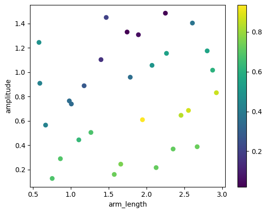
The results include the full S matrix for each crossing variation. To help us make sense of all this data, we can define a figure of merit for the design and plot it versus the crossing parameters. In this case, a reasonable definition is to use the minimal transmission value within the frequency range we’re interested in. Let’s first create a result table with only the parameters and our figure of merit, instead of the whole S matrix objects:

names = [v.name for v in variables]
table = np.array([(*v, np.abs(s["P0@0", "P2@0"]).min() ** 2) for *v, s in results])
table

array([[1.89293245, 1.30670413, 0.05502584],
       [1.78530457, 0.95793781, 0.34759576],
       [1.57431442, 0.15939063, 0.73172939],
       [1.39931042, 1.10239893, 0.15510817],
       [1.74379972, 1.32907849, 0.02096373],
       [0.66835153, 0.56466724, 0.42346457],
       [2.07250101, 1.05543504, 0.49904752],
       [2.45512328, 0.64501438, 0.83864492],
       [2.55332675, 0.68507742, 0.87208878],
       [2.12682069, 0.21543469, 0.71893195],
       [0.98118614, 0.76343902, 0.34506908],
       [2.66823248, 0.38698483, 0.72716119],
       [1.46807783, 1.44878793, 0.2012137 ],
       [1.94662566, 0.60877627, 0.9361136 ],
       [2.92168546, 0.83047987, 0.86310329],
       [2.35086521, 0.36836535, 0.71462285],
       [0.86364256, 0.28845985, 0.68888216],
       [2.24903115, 1.48379688, 0.02435246],
       [2.26344246, 1.15381968, 0.54550564],
       [2.87219256, 1.0157638 , 0.60485237],
       [0.59253126, 0.90813608, 0.42837409],
       [1.26638186, 0.50425125, 0.67812875],
       [1.00809177, 0.73810412, 0.33855038],
       [0.58137162, 1.24378247, 0.4852113 ],
       [2.80040379, 1.17426609, 0.5555673 ],
       [1.10690058, 0.44344074, 0.63456104],
       [1.17656064, 0.88775554, 0.273729  ],
       [0.75534563, 0.12637548, 0.68102564],
       [2.60544912, 1.4027804 , 0.37433997],
       [1.66009647, 0.24387858, 0.7518179 ]])

plt.scatter(table[:, 0], table[:, 1], c=table[:, 2])
plt.xlabel(names[0])
plt.ylabel(names[1])
_ = plt.colorbar()

Local Optimization

We use scipy to optimize the crossing around the best result we found through the Nelder-Mead method, which does not require a gradient computation. More advanced optimization methods based on ajoint computations are available in Tidy3D directly, if the device require those due to, for example, a large number of parameters.

The only step required to run the optimization is the creation of an objective function to be minimized. It receives arguments as an array, which we decompose into the 2 parameters for our crossing. Furthermore, because we desire to maximize the minimal transmission, we use a negative sign in our figure of merit:

def objective(args):
    kwargs = dict(zip(names, args))
    c = sine_crossing(**kwargs)
    s_matrix = c.s_matrix(freqs)
    min_transmission = np.abs(s_matrix["P0@0", "P2@0"]).min() ** 2

    # We can print the current evaluation result to keep track of the optimization process
    print(args, "→", min_transmission, flush=True)

    return -min_transmission

For the actual optimization run, we limit the convergence tolerances to reasonable values, as well as the number of function evaluations so that we don’t run unnecessary simulations. If those values end up being too small, we can always restart the optimization from the last best parameters.

best_variation = np.argmax(table[:, 2])
initial_guess = (table[best_variation, 0], table[best_variation, 1])

opt_result = scipy.optimize.minimize(
    objective,
    initial_guess,
    method="Nelder-Mead",
    bounds=[v.value_spec["value_range"] for v in variables],
    options={"maxfev": 16, "fatol": 0.005, "xatol": 0.005},
)
opt_result

Starting...
Progress: 100%
[1.94662566 0.60877627] → 0.9361136041097525
Starting...
Progress: 100%
[2.04395694 0.60877627] → 0.9355843931070496
Starting...
Progress: 100%
[1.94662566 0.63921508] → 0.9055909384723156
Starting...
Progress: 100%
[2.04395694 0.57833745] → 0.9207131107240649
Starting...
Progress: 100%
[2.01962412 0.59355686] → 0.9341204906973903
Starting...
Progress: 100%
[1.97095848 0.62399567] → 0.9241946488375885
Starting...
Progress: 100%
[2.00745771 0.60116656] → 0.9390136991334345
Starting...
Progress: 100%
[1.91012643 0.60116656] → 0.9367254347539961
Starting...
Progress: 100%
[1.97095848 0.59355686] → 0.9388670877968563
Starting...
Progress: 100%
[2.06828976 0.59355686] → 0.9225676810839387
Starting...
Progress: 100%
[1.94966726 0.59926414] → 0.9402911659541455
Starting...
Progress: 100%
[1.98616649 0.60687384] → 0.9403413233494465
Starting...
Progress: 100%
[1.9937705  0.61353233] → 0.9370608560536259
Starting...
Progress: 100%
[1.92837604 0.60497142] → 0.9361766077689085
Starting...
Progress: 100%
[1.98768729 0.60211778] → 0.9412344631728908
Starting...
Progress: 100%
[2.02418652 0.60972748] → 0.9382037516805125

       message: Maximum number of function evaluations has been exceeded.
       success: False
        status: 1
           fun: -0.9412344631728908
             x: [ 1.988e+00  6.021e-01]
           nit: 8
          nfev: 16
 final_simplex: (array([[ 1.988e+00,  6.021e-01],
                       [ 1.986e+00,  6.069e-01],
                       [ 1.950e+00,  5.993e-01]]), array([-9.412e-01, -9.403e-01, -9.403e-01]))

Inspecting the Optimized Component

We can recreate the best variation for out technology and reset its model to remove the helper symmetries and include a field monitor if we want to fully inspect the component. Of course, with our parameters being layout dimensions, we should not use an arbitrary number of decimals, so we round them appropriately: in this case, 2 decimals (10 nm grid) should suffice.

kwargs = dict(zip(names, np.round(opt_result.x, decimals=2)))

crossing = sine_crossing(**kwargs)

tidy3d_model = pf.Tidy3DModel(
    monitors=[
        td.FieldMonitor(
            name="field",
            center=(0, 0, 0.11),
            size=(td.inf, td.inf, 0),
            freqs=[freqs.mean()],
        )
    ]
)

crossing.add_model(tidy3d_model, "Tidy3D")

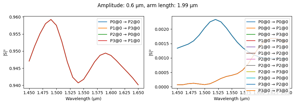
s_matrix = crossing.s_matrix(freqs)
fig, ax = pf.plot_s_matrix(s_matrix)
_ = fig.suptitle(f"Amplitude: {kwargs['amplitude']} μm, arm length: {kwargs['arm_length']} μm")

Starting...
Loading cached simulation from .tidy3d/pf_cache/LUS/fdtd_info-QDH4AZRXVOTRUIUD33ZFA766RDKHYUJT47SI56G4XRBVWPSFGLKA.json.
Loading cached simulation from .tidy3d/pf_cache/LUS/fdtd_info-J4Y46LDP32VSJI34VKOEZ2SEHTUY3DJJ7JSVZS6GPSANKMNP7NAA.json.
Loading cached simulation from .tidy3d/pf_cache/LUS/fdtd_info-2HOIKI6GJ3BH3PKLRBWY7LSNELZIEODE2247TF3ZSCE2NG7QGYBQ.json.
Loading cached simulation from .tidy3d/pf_cache/LUS/fdtd_info-KGELYV7KALAMIAZQCYC4Y6ENEHE2C7I7LOZYZKBKDR5OHBW73YGA.json.
Progress: 100%

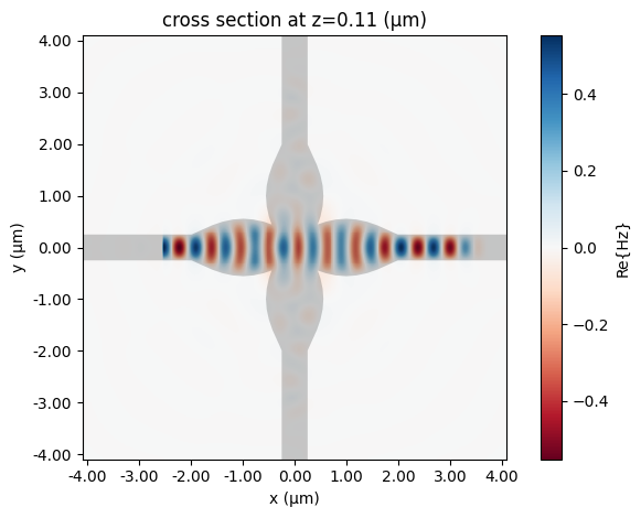
In order to plot the fields, we can use the batch_data_for function from the Tidy3D model to get the BatchData that includes the fields from our extra monitor:

sim_data = tidy3d_model.batch_data_for(crossing)
_ = sim_data["P0@0"].plot_field("field", "Hz", robust=False)