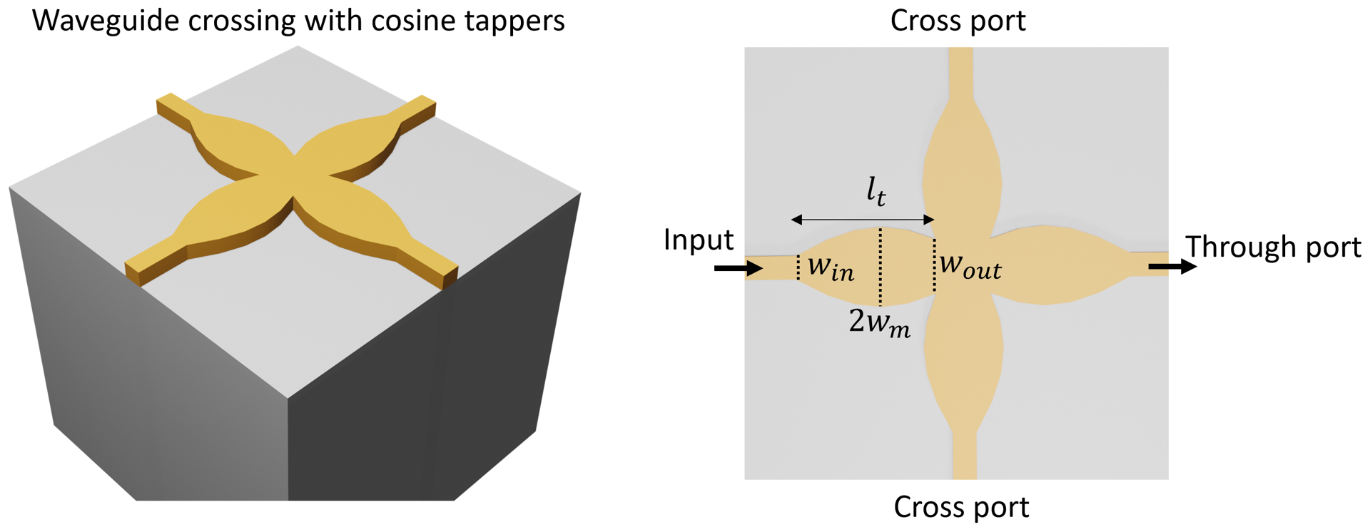
Waveguide crossing based on cosine tapers#
To achieve a high integration density on a photonic chip, efficient routing of light with low loss using compact junctions is necessary. Therefore, waveguide crossings are crucial building blocks in high performance integrated circuits.
This example model demonstrates the simulation of a waveguide crossing based on cosine tapers. The convex cosine taper focuses the guided mode at the center of the crossing junction. This ensures the light is efficiently transmitted into the through port instead of scattered into the cross ports. The device achieves an insertion loss of ~0.2 dB and crosstalk ~-30 dB in the O-band (1260 nm -1360 nm). The design is adapted from Sujith Chandran, et al. “Beam shaping for ultra-compact waveguide crossings on monolithic silicon photonics platform,” Opt. Lett. 45, 6230-6233 (2020).
If you are new to the finite-difference time-domain (FDTD) method, we highly recommend going through our FDTD101 tutorials. For more simulation examples, please visit our examples page. FDTD simulations can diverge due to various reasons. If you run into any simulation divergence issues, please follow the steps outlined in our troubleshooting guide to resolve it.
[1]:
import matplotlib.pyplot as plt
import numpy as np
import tidy3d as td
import tidy3d.web as web
from scipy.optimize import fsolve
Simulation Setup#
Define geometric parameters and materials. In this device, the Si waveguide has a thickness of 161 nm and a width of 350 nm.
[2]:
h = 0.161  # waveguide thickness
w_in = 0.35  # input taper width
w_out = 1.1  # output taper width
w_m = 0.75  # amplitude of the cos function
l_t = 5.3  # taper length
inf_eff = 1000  # effective infinity used to make sure the waveguides extend into the pml
[3]:
si = td.Medium(permittivity=3.67**2)
sio2 = td.Medium(permittivity=1.45**2)
The taper width is described by a cosine function \(w(x)=w_m cos(ax+b)\). To determine the parameters \(a\) and \(b\), we solve a system of equations to ensure \(w(x)=w_{in}/2\) at the beginning of the taper and \(w(x)=w_{out}/2\) at the end of the taper. This can be easily done using fsolve from Scipy.
After we obtain \(w(x)\), vertices can be generated and the taper can be made using PolySlab. Once the first taper is made, the rest three tapers can be made by manipulating the vertices with the symmetry relation.
[4]:
# numerically solve for the cos function that describes the taper shape
def equations(x0):
    a, b = x0
    return (
        w_m * np.cos(a * (-w_out / 2) + b) - w_out / 2,
        w_m * np.cos(a * (-w_out / 2 - l_t) + b) - w_in / 2,
    )


a, b = fsolve(equations, (0.5, 2))

x = np.linspace(-w_out / 2 - l_t, -w_out / 2, 30)
w = w_m * np.cos(a * x + b)

# using the calculated taper shape to construct the taper as a PolySlab
vertices = np.zeros((2 * len(x), 2))
vertices[:, 0] = np.concatenate((x, np.flipud(x)))
vertices[:, 1] = np.concatenate((w, -np.flipud(w)))
taper_1 = td.Structure(
    geometry=td.PolySlab(vertices=vertices, axis=2, slab_bounds=(-h / 2, h / 2)),
    medium=si,
)

# creating the other four tapers by manipulating the vertices of the first taper
vertices = np.array(vertices)
vertices[:, 0] = -vertices[:, 0]
taper_2 = td.Structure(
    geometry=td.PolySlab(vertices=vertices, axis=2, slab_bounds=(-h / 2, h / 2)),
    medium=si,
)

vertices = np.array(vertices)
vertices[:, [1, 0]] = vertices[:, [0, 1]]
taper_3 = td.Structure(
    geometry=td.PolySlab(vertices=vertices, axis=2, slab_bounds=(-h / 2, h / 2)),
    medium=si,
)

vertices = np.array(vertices)
vertices[:, 1] = -vertices[:, 1]
taper_4 = td.Structure(
    geometry=td.PolySlab(vertices=vertices, axis=2, slab_bounds=(-h / 2, h / 2)),
    medium=si,
)

# creating the center crossing junction using a Box
corner = 0
center = td.Structure(
    geometry=td.Box.from_bounds(
        rmin=(-w_out / 2 - corner, -w_out / 2 - corner, -h / 2),
        rmax=(w_out / 2 + corner, w_out / 2 + corner, h / 2),
    ),
    medium=si,
)

# creating the input port and through port
horizontal_wg = td.Structure(
    geometry=td.Box.from_bounds(
        rmin=(-inf_eff, -w_in / 2, -h / 2), rmax=(inf_eff, w_in / 2, h / 2)
    ),
    medium=si,
)

# creating the cross ports
vertical_wg = td.Structure(
    geometry=td.Box.from_bounds(
        rmin=(-w_in / 2, -inf_eff, -h / 2), rmax=(w_in / 2, inf_eff, h / 2)
    ),
    medium=si,
)
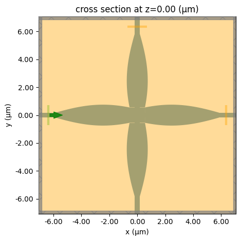
Set up simulation domain, source, and monitors. A mode source is used to excite the input waveguide. A field monitor at \(z=0\) plane is added to monitor the field propagation. Two flux monitors are added at the through port and cross port to monitor the transmission and crosstalk levels.
Before running the simulation, we can use the plot method to ensure the geometry, source, and monitors are set up correctly.
[5]:
lda0 = 1.31  # central wavelength
freq0 = td.C_0 / lda0  # operation frequency
ldas = np.linspace(1.26, 1.36, 101)  # wavelength range of interest
freqs = td.C_0 / ldas  # frequency range of interest

l_wg = 1  # input/output waveguide length
Lx = 2 * l_t + w_out + 2 * l_wg
Ly = 2 * l_t + w_out + 2 * l_wg
Lz = 1.5 * lda0
sim_size = (Lx, Ly, Lz)

# define a mode source for excitation using the lowest order mode
mode_source = td.ModeSource(
    center=(-Lx / 2 + l_wg / 2, 0, 0),
    size=(0, 4 * w_in, 4 * h),
    source_time=td.GaussianPulse(freq0=freq0, fwidth=freq0 / 10),
    direction="+",
    mode_spec=td.ModeSpec(
        num_modes=1,
        target_neff=3.455,
        sort_spec=td.ModeSortSpec(
            filter_key="TE_fraction", filter_order="over", filter_reference=0.5
        ),
    ),
    mode_index=0,
)

# add a field monitor at z=0 for field visualization
field_monitor = td.FieldMonitor(
    center=(0, 0, 0), size=(td.inf, td.inf, 0), freqs=[freq0], name="field"
)

# define a flux monitor to detect transmission to the through port
flux_monitor_through = td.FluxMonitor(
    center=(Lx / 2 - l_wg / 2, 0, 0),
    size=(0, 4 * w_in, 4 * h),
    freqs=freqs,
    name="flux_through",
)

# define a flux monitor to detect transmission to the cross port
flux_monitor_cross = td.FluxMonitor(
    center=(0, Ly / 2 - l_wg / 2, 0),
    size=(4 * w_in, 0, 4 * h),
    freqs=freqs,
    name="flux_cross",
)

sim = td.Simulation(
    center=(0, 0, 0),
    size=sim_size,
    grid_spec=td.GridSpec.auto(min_steps_per_wvl=20, wavelength=lda0),
    structures=[taper_1, taper_2, taper_3, taper_4, center, horizontal_wg, vertical_wg],
    sources=[mode_source],
    monitors=[field_monitor, flux_monitor_through, flux_monitor_cross],
    run_time=1e-12,
    boundary_spec=td.BoundarySpec.all_sides(boundary=td.PML()),
    medium=sio2,
)

sim.plot(z=0)
plt.show()
To have a better visualization, we can also plot the simulation in 3D.
[6]:
sim.plot_3d()
Once the simulation set up is verified, submit job to the server. Before running the simulation, we can get a cost estimation using estimate_cost. This prevents us from accidentally running large jobs that we set up by mistake. The estimated cost is the maximum cost corresponding to running all the time steps.
[7]:
job = web.Job(simulation=sim, task_name="waveguide_crossing", verbose=True)
estimated_cost = web.estimate_cost(job.task_id)
14:01:33 UTC Created task 'waveguide_crossing' with resource_id
             'fdve-e3b21982-f5f4-424c-910d-f722c263fec5' and task_type 'FDTD'.
             View task using web UI at
             'https://tidy3d.simulation.cloud/workbench?taskId=fdve-e3b21982-f5f
             4-424c-910d-f722c263fec5'.
Task folder: 'default'.
14:01:56 UTC Estimated FlexCredit cost: 0.492. Minimum cost depends on task
             execution details. Use 'web.real_cost(task_id)' to get the billed
             FlexCredit cost after a simulation run.
The cost is reasonably so we can run the simulation.
[8]:
sim_data = job.run(path="data/simulation_data.hdf5")
14:02:05 UTC Estimated FlexCredit cost: 0.492. Minimum cost depends on task
             execution details. Use 'web.real_cost(task_id)' to get the billed
             FlexCredit cost after a simulation run.
14:02:06 UTC status = queued
             To cancel the simulation, use 'web.abort(task_id)' or
             'web.delete(task_id)' or abort/delete the task in the web UI.
             Terminating the Python script will not stop the job running on the
             cloud.
14:02:18 UTC status = preprocess
14:02:23 UTC starting up solver
14:02:24 UTC running solver
14:02:48 UTC early shutoff detected at 56%, exiting.
status = postprocess
14:02:52 UTC status = success
14:02:54 UTC View simulation result at
             'https://tidy3d.simulation.cloud/workbench?taskId=fdve-e3b21982-f5f
             4-424c-910d-f722c263fec5'.
14:03:04 UTC Loading results from data/simulation_data.hdf5
             WARNING: Warning messages were found in the solver log. For more
             information, check 'SimulationData.log' or use
             'web.download_log(task_id)'.
Result Visualization#
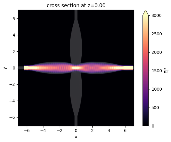
After the simulation is complete, first plot the field intensity distribution.
From the figure below, a good transmission to the through port is observed. In the crossing junction, a strong field focus is formed due to the focusing property of the cosine taper.
[9]:
sim_data.plot_field(
    field_monitor_name="field", field_name="E", val="abs^2", f=freq0, vmin=0, vmax=3000
)
plt.show()
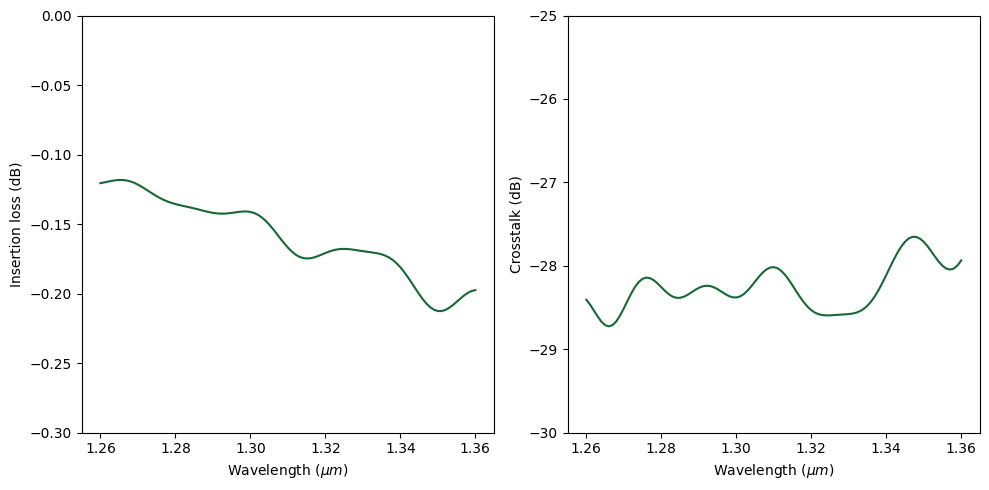
Finally, to quantify the designed waveguide crossing’s performance, plot insertion loss and crosstalk level.
[10]:
f, (ax1, ax2) = plt.subplots(1, 2, tight_layout=True, figsize=(10, 5))

T_through = sim_data["flux_through"].flux
T_cross = sim_data["flux_cross"].flux

ax1.plot(ldas, 10 * np.log10(T_through))
ax1.set_xlabel(r"Wavelength ($\mu m$)")
ax1.set_ylabel("Insertion loss (dB)")
ax1.set_ylim((-0.3, 0))

ax2.plot(ldas, 10 * np.log10(T_cross / T_through))
ax2.set_xlabel(r"Wavelength ($\mu m$)")
ax2.set_ylabel("Crosstalk (dB)")
ax2.set_ylim((-30, -25))
plt.show()
[ ]: