Build a simple waveguide bend simulator GUI#
A case study of a 90-degree waveguide bend simulator#
Tidy3D offers a versatile web-based graphical user interface (GUI) suitable for a wide range of FDTD simulations from photonic integrated circuit components to metasurfaces and diffractive gratings. While this general-purpose GUI is beneficial for its extensive capabilities, there are situations where you might need to focus on simulating a specific device type repeatedly. For these scenarios, Tidy3D’s Python
API paired with open-source Python libraries such as tkinter enables the easy creation of a customized GUI. This specialized interface, designed with fewer controls and buttons, streamlines the simulation process for ease of use. By sharing this bespoke GUI with less experienced colleagues, they can also efficiently run simulations without extensive prior knowledge or
expertise in FDTD.
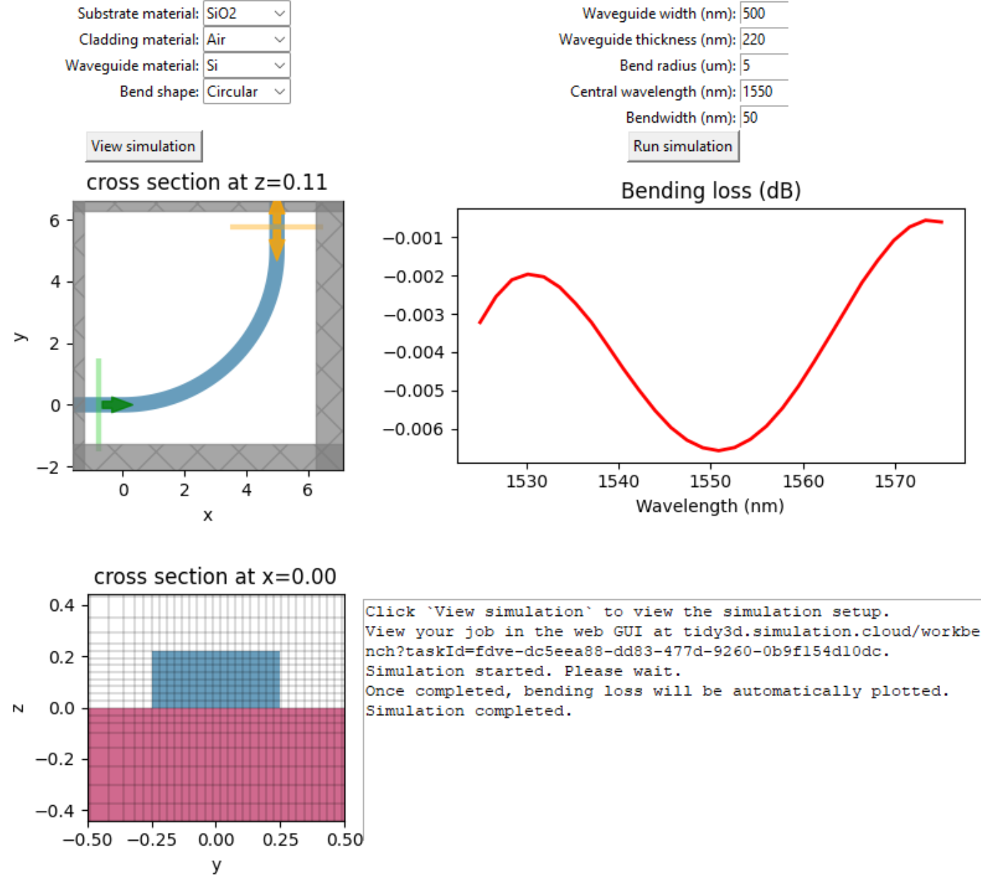
Here we demonstrate the creation of a simple GUI for 90-degree waveguide bend simulation. In this GUI, users can select materials for the waveguide bend, substrate, and cladding through combo boxes. We include common materials such as silicon, silicon nitride, silicon oxide, and so on. Users can also select between a circular bend and an Euler bend. Geometric parameters can be entered in the input boxes to define the waveguide dimensions and bend radius. Before running the simulation, users can view the simulation setup as well as the grid by clicking the “View simulation” button. Lastly, users can start the simulation by clicking the “Run simulation” button. After the simulation, the bending loss is automatically plotted. We also include a text window to display some relevant text outputs.
As a tutorial, we use Jupyter Notebook to store the codes for the GUI creation. If you run the notebook, the GUI window will appear and you can interact with it. One can further package this GUI into a stand-alone application for easier distribution if needed. The GUI should look like below after launching it:
To run this notebook successfully, one needs to have the tkinter, gdstk, and other relevant libraries installed. First, we perform the necessary Python library imports.
[1]:
import tkinter as tk
from tkinter import ttk

import gdstk
import matplotlib.pyplot as plt
import numpy as np
import scipy.integrate as integrate
import tidy3d as td
import tidy3d.web as web
from matplotlib.backends.backend_tkagg import FigureCanvasTkAgg
from scipy.optimize import fsolve
Define basic parameters. These parameters are not meant to be changed by the GUI user.
[2]:
num_freq = 30  # number of frequency points
num_theta = 100  # number of circular bend points
nm_to_um = 1e-3  # conversion factor from nm to um
min_steps_per_wvl = 15  # grid resolution

# euler bend parameters
R_eff = 4
A = 2.4
We put the supported media into a dictionary for easier mapping later on. In this specific GUI, we include a few common materials such as silicon, silicon dioxide, silicon nitride, and so on. More can be included as needed.
Two waveguide bend shapes are included: circular or Euler.
[3]:
# dictionary to store all materials
media = {
    "Si": td.material_library["cSi"]["Palik_Lossless"],
    "SiO2": td.material_library["SiO2"]["Palik_Lossless"],
    "Si3N4": td.material_library["Si3N4"]["Luke2015PMLStable"],
    "Air": td.Medium(permittivity=1),
    "PMMA": td.material_library["PMMA"]["Horiba"],
    "InAs": td.material_library["InAs"]["Palik"],
    "GaAs": td.material_library["GaAs"]["Palik_Lossy"],
}

materials = list(media.keys())  # list of materials for the combo box
shapes = ["Circular", "Euler"]  # list of shapes for the combo box
Next we define functions to compute the coordinates for the circular and Euler bends. Many codes here are adapted from our previous example on Euler waveguide bends.
[4]:
# function to calculate the coordinates for a circular bend
def circular_xy(r):
    theta = np.linspace(0, np.pi / 2, num_theta)
    x_circle = r * np.sin(theta)
    y_circle = r - r * np.cos(theta)
    return x_circle, y_circle


# function to calculate the coordinates for an Euler bend
def euler_xy(r):
    L_max = 0  # starting point of L_max
    precision = 0.05  # increment of L_max at each iteration
    tolerance = 0.01  # difference tolerance of the derivatives

    # determine L_max
    while True:
        L_max = L_max + precision  # update L_max
        Ls = np.linspace(0, L_max, 50)  # L at (x1,y1)
        x1 = np.zeros(len(Ls))  # x coordinate of the clothoid curve
        y1 = np.zeros(len(Ls))  # y coordinate of the clothoid curve

        # compute x1 and y1 using the above integral equations
        for i, L in enumerate(Ls):
            y1[i], err = integrate.quad(lambda theta: A * np.sin(theta**2 / 2), 0, L / A)
            x1[i], err = integrate.quad(lambda theta: A * np.cos(theta**2 / 2), 0, L / A)

        # compute the derivative at L_max
        k = -(x1[-1] - x1[-2]) / (y1[-1] - y1[-2])
        xp = x1[-1]
        yp = y1[-1]
        # check if the derivative is continuous at L_max
        R = np.sqrt(
            ((R_eff + k * xp - yp) / (k + 1) - xp) ** 2
            + (-(R_eff + k * xp - yp) / (k + 1) + R_eff - yp) ** 2
        )
        if np.abs(R - A**2 / L_max) < tolerance:
            break

    # after L_max is determined, R_min is also determined
    R_min = A**2 / L_max

    x3 = np.flipud(R_eff - y1)
    y3 = np.flipud(R_eff - x1)

    # solve for the parameters of the circular curve
    def circle(var):
        a = var[0]
        b = var[1]
        Func = np.empty(2)
        Func[0] = (xp - a) ** 2 + (yp - b) ** 2 - R_min**2
        Func[1] = (R_eff - yp - a) ** 2 + (R_eff - xp - b) ** 2 - R_min**2
        return Func

    a, b = fsolve(circle, (0, R_eff))

    # calculate the coordinates of the circular curve
    x2 = np.linspace(xp + 0.01, R_eff - yp - 0.01, 50)
    y2 = -np.sqrt(R_min**2 - (x2 - a) ** 2) + b

    x_euler = np.concatenate((x1, x2, x3))
    y_euler = np.concatenate((y1, y2, y3))

    return r * x_euler / R_eff, r * y_euler / R_eff
We also create a helper function to convert the \(x\) and \(y\) coordinates of a path into a Tidy3D Structure by utilizing gdstk.
[5]:
# function to convert the coordinates of a path into a bend structure
def line_to_structure(x, y, r, t, w, wg_mat):
    cell = gdstk.Cell("bend")  # define a gds cell
    inf_eff = 2 * r
    # add points to include the input and output straight waveguides
    x = np.insert(x, 0, -inf_eff)
    x = np.append(x, r)
    y = np.insert(y, 0, 0)
    y = np.append(y, inf_eff)

    cell.add(gdstk.FlexPath(x + 1j * y, w, layer=1, datatype=0))  # add path to cell

    # define structure from cell
    bend = td.Structure(
        geometry=td.PolySlab.from_gds(
            cell,
            gds_layer=1,
            axis=2,
            slab_bounds=(0, t),
        )[0],
        medium=media[wg_mat],
    )
    return bend
Next we define a function to create a Tidy3D Simulation instance. In this function, we need to extract the values of the user inputs in the GUI, define the waveguide bend structure based on the extracted values, define a ModeSource to excite the input waveguide and a ModeMonitor to measure the transmission to the output waveguide, and lastly return a Simulation.
[6]:
# function to compute wavelength range
def get_ldas():
    lda0 = float(lda0_box.get()) * nm_to_um
    bw = float(bw_box.get()) * nm_to_um
    ldas = np.linspace(lda0 - 0.5 * bw, lda0 + 0.5 * bw, num_freq)
    return lda0, ldas


# function to define the bend simulation
def make_sim():
    # get user input values from the gui
    sub_mat = substrate_box.get()
    wg_mat = wg_box.get()
    clad_mat = cladding_box.get()
    r = float(radius_box.get())
    t = float(thickness_box.get()) * nm_to_um
    w = float(width_box.get()) * nm_to_um
    shape = shape_box.get()

    # define simulation wavelength range
    lda0, ldas = get_ldas()
    freq0 = td.C_0 / lda0
    freqs = td.C_0 / ldas
    fwidth = 0.5 * (np.max(freqs) - np.min(freqs))

    # create structures
    if shape == "Circular":
        x, y = circular_xy(r)
    elif shape == "Euler":
        x, y = euler_xy(r)

    bend = line_to_structure(x, y, r, t, w, wg_mat)

    sub = td.Structure(
        geometry=td.Box.from_bounds(rmin=(-2 * r, -2 * r, -2 * r), rmax=(2 * r, 2 * r, 0)),
        medium=media[sub_mat],
    )

    # define source and monitor
    target_neff = media[wg_mat].nk_model(freq0)[0]
    mode_spec = td.ModeSpec(num_modes=1, target_neff=target_neff)
    mode_source = td.ModeSource(
        center=(-lda0 / 2, 0, t / 2),
        size=(0, 6 * w, 8 * t),
        source_time=td.GaussianPulse(freq0=freq0, fwidth=fwidth),
        direction="+",
        mode_spec=mode_spec,
        mode_index=0,
    )

    # add a mode monitor to measure transmission
    mode_monitor = td.ModeMonitor(
        center=(r, r + lda0 / 2, t / 2),
        size=(6 * w, 0, 8 * t),
        freqs=freqs,
        mode_spec=mode_spec,
        name="mode",
    )

    run_time = 15 * np.pi * r / td.C_0  # simulation run time

    # define simulation
    sim = td.Simulation(
        center=(r / 2, r / 2, t / 2),
        size=(r + 2 * w + lda0, r + 2 * w + lda0, 2 * lda0),
        grid_spec=td.GridSpec.auto(min_steps_per_wvl=min_steps_per_wvl, wavelength=lda0),
        structures=[bend, sub],
        sources=[mode_source],
        monitors=[mode_monitor],
        run_time=run_time,
        boundary_spec=td.BoundarySpec.all_sides(boundary=td.PML()),
        medium=media[clad_mat],
    )
    return sim
Lastly, we need to define a few more functions to visualize the simulation, run the simulation, and plot the simulation result.
[7]:
# function to plot the simulation cross sections as well as the grid
def plot_sim():
    t = float(thickness_box.get()) * nm_to_um
    w = float(width_box.get()) * nm_to_um

    sim = make_sim()
    ax1.clear()
    sim.plot(z=t / 2, ax=ax1)
    xy_canvas.draw()

    ax3.clear()
    sim.plot(x=0, ax=ax3)
    sim.plot_grid(x=0, ax=ax3)
    ax3.set_xlim(-w, w)
    ax3.set_ylim(-2 * t, 2 * t)
    yz_canvas.draw()


# function to run the simulation
def run_sim():
    ax2.clear()
    result_canvas.draw()
    sim = make_sim()
    job = web.Job(simulation=sim, task_name="Bend")
    text_widget.insert(
        "end",
        "View your job in the web GUI at "
        + f"tidy3d.simulation.cloud/workbench?taskId={job.task_id}.\n",
    )
    text_widget.insert("end", "Simulation started. Please wait.\n")
    text_widget.insert("end", "Once completed, bending loss will be automatically plotted.\n")
    text_widget.see(tk.END)
    root.update_idletasks()
    sim_data = job.run()
    text_widget.insert("end", "Simulation completed.\n")
    text_widget.see(tk.END)

    return sim_data


# function to plot the simulation result
def plot_result():
    _, ldas = get_ldas()
    sim_data = run_sim()
    amp = sim_data["mode"].amps.sel(mode_index=0, direction="+")
    T = np.abs(amp) ** 2

    ax2.plot(ldas / nm_to_um, 10 * np.log10(T), c="red", linewidth=2)
    ax2.set_title("Bending loss (dB)")
    ax2.set_xlabel("Wavelength (nm)")
    result_canvas.draw()
With all the preparation works ready, we can go ahead and start our GUI layout design.
[8]:
# Set up the main window
root = tk.Tk()
root.title("90 degree bend simulator")
root.configure(bg="white")
root.resizable(False, False)

# add a combo box for substrate material selection
substrate_label = tk.Label(root, text="Substrate material:", bg="white")
substrate_label.grid(column=0, row=0, sticky="E")
substrate_box = ttk.Combobox(root, values=materials, width=8)
substrate_box.grid(column=1, row=0, sticky="W")
substrate_box.current(1)

# add a combo box for cladding material selection
cladding_label = tk.Label(root, text="Cladding material:", bg="white")
cladding_label.grid(column=0, row=1, sticky="E")
cladding_box = ttk.Combobox(root, values=materials, width=8)
cladding_box.grid(column=1, row=1, sticky="W")
cladding_box.current(3)

# add a combo box for waveguide material selection
wg_label = tk.Label(root, text="Waveguide material:", bg="white")
wg_label.grid(column=0, row=2, sticky="E")
wg_box = ttk.Combobox(root, values=materials, width=8)
wg_box.grid(column=1, row=2, sticky="W")
wg_box.current(0)

# add a combo box for bend shape selection
shape_label = tk.Label(root, text="Bend shape:", bg="white")
shape_label.grid(column=0, row=3, sticky="E")
shape_box = ttk.Combobox(root, values=shapes, width=8)
shape_box.grid(column=1, row=3, sticky="W")
shape_box.current(0)

# add a label and a input box for waveguide width
width_label = tk.Label(root, text="Waveguide width (nm):", bg="white")
width_label.grid(column=2, row=0, sticky="E")
width_box = tk.Entry(root, width=6)
width_box.grid(column=3, row=0, sticky="W")
width_box.insert(0, "500")

# add a label and a input box for waveguide thickness
thickness_label = tk.Label(root, text="Waveguide thickness (nm):", bg="white")
thickness_label.grid(column=2, row=1, sticky="E")
thickness_box = tk.Entry(root, width=6)
thickness_box.grid(column=3, row=1, sticky="W")
thickness_box.insert(0, "220")

# add a label and a input box for waveguide radius
radius_label = tk.Label(root, text="Bend radius (um):", bg="white")
radius_label.grid(column=2, row=2, sticky="E")
radius_box = tk.Entry(root, width=6)
radius_box.grid(column=3, row=2, sticky="W")
radius_box.insert(0, "5")

# add a label and a input box for central wavelength
lda0_label = tk.Label(root, text="Central wavelength (nm):", bg="white")
lda0_label.grid(column=2, row=3, sticky="E")
lda0_box = tk.Entry(root, width=6)
lda0_box.grid(column=3, row=3, sticky="W")
lda0_box.insert(0, "1550")

# add a label and a input box for bandwidth
bw_label = tk.Label(root, text="Bandwidth (nm):", bg="white")
bw_label.grid(column=2, row=4, sticky="E")
bw_box = tk.Entry(root, width=6)
bw_box.grid(column=3, row=4, sticky="W")
bw_box.insert(0, "50")

# add a button for viewing simulation
view_button = tk.Button(root, text="View simulation", command=plot_sim)
view_button.grid(column=0, row=5, sticky="E")

# add a button for running simulation
run_button = tk.Button(root, text="Run simulation", command=plot_result)
run_button.grid(column=2, row=5, sticky="E")

# add a plot for xy cross section
fig1, ax1 = plt.subplots(figsize=(3, 3), tight_layout=True)
xy_canvas = FigureCanvasTkAgg(fig1, master=root)
xy_canvas_widget = xy_canvas.get_tk_widget()
xy_canvas_widget.grid(column=0, row=6, columnspan=2)
plt.close(fig1)

# add a plot for bending loss spectrum
fig2, ax2 = plt.subplots(figsize=(5, 3), tight_layout=True)
result_canvas = FigureCanvasTkAgg(fig2, master=root)
result_canvas_widget = result_canvas.get_tk_widget()
result_canvas_widget.grid(column=2, row=6, columnspan=2)
plt.close(fig2)

# add a plot for yz cross section
fig3, ax3 = plt.subplots(figsize=(3, 3), tight_layout=True)
yz_canvas = FigureCanvasTkAgg(fig3, master=root)
yz_canvas_widget = yz_canvas.get_tk_widget()
yz_canvas_widget.grid(column=0, row=7, columnspan=2)
plt.close(fig3)

# add a text box to display information
text_widget = tk.Text(root, height=12, width=1)
text_widget.grid(column=2, row=7, columnspan=2, sticky="ew")
default_text = "Click `View simulation` to view the simulation setup.\n"
text_widget.insert("1.0", default_text)
With everything ready, we can now launch the GUI.
[9]:
root.mainloop()
In conclusion, this notebook demonstrates how to make a simple purpose-specific GUI for Tidy3D. By following this workflow, users have the full freedom to create GUIs that suit their particular workflow and experience level. More complex features and visualizations can be implemented to further enhance the usability of the GUI if desired. Simple GUIs are a great way to get inexperienced users around you to get started with Tidy3D.
For easier distribution, one can package this GUI into a stand-alone executable following tutorials such as here.
[ ]: