Waveguide bragg gratings#
Bragg gratings are often used in waveguides, such as optical fibres, which can reflect light of certain frequencies while transmitting others. This is typically achieved by periodically changing the refractive index or dielectric constant in a section of the waveguide, and the reflective and transmitting frequency bands are controlled by appropriately designing the periodicity and material or geometry parameters of the grating.
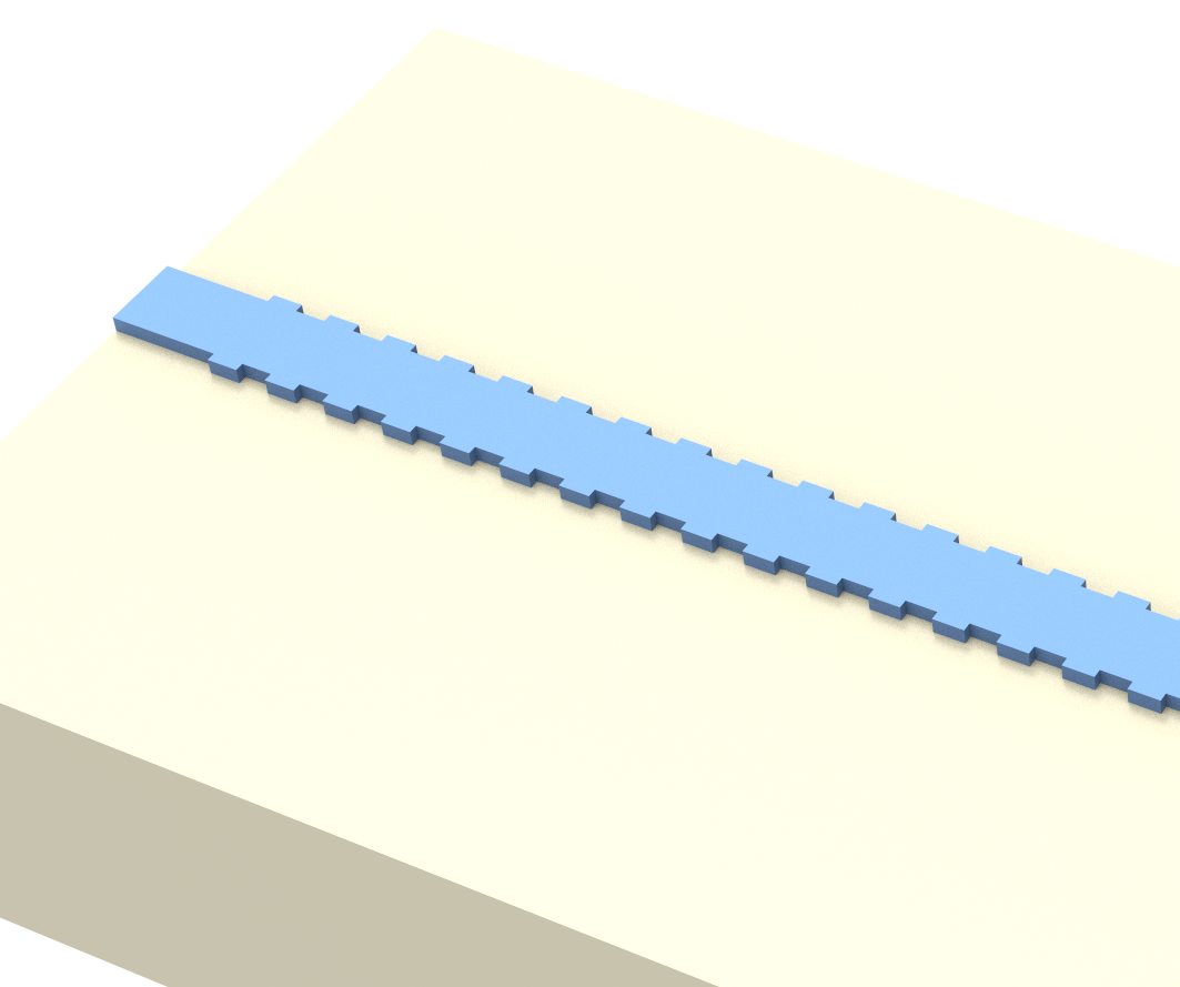
In this example, sections of two Bragg gratings will be simulated. The first one involves a waveguide with a perfectly aligned corrugation on either side, which causes it to act as a reflector. The second one is similar, but with the corrugation on one side misaligned with the corrugation on the other side, so that the structure primarily transmits power.
Reference: Xu Wang, Yun Wang, Jonas Flueckiger, Richard Bojko, Amy Liu, Adam Reid, James Pond, Nicolas A. F. Jaeger, and Lukas Chrostowski, "Precise control of the coupling coefficient through destructive interference in silicon waveguide Bragg gratings," Opt. Lett. 39, 5519-5522 (2014), DOI: 10.1364/OL.39.005519.
As a relevant example, please see the distributed Bragg reflector. For more integrated photonic examples such as the 8-Channel mode and polarization de-multiplexer, the broadband bi-level taper polarization rotator-splitter, and the broadband directional coupler, please visit our examples page.
If you are new to the finite-difference time-domain (FDTD) method, we highly recommend going through our FDTD101 tutorials.
[1]:
# basic imports
import matplotlib.pylab as plt
import numpy as np

# Tidy3D imports
import tidy3d as td
Structure Setup#
First, the geometry of the structure is defined. Both waveguides are set up in the same simulation side-by-side.
[2]:
# materials
Air = td.Medium(permittivity=1.0)
Si = td.Medium(permittivity=3.47**2)
SiO2 = td.Medium(permittivity=1.44**2)

# geometric parameters
wg_height = 0.22
wg_feed_length = 0.75
wg_feed_width = 0.5
corrug_width = 0.05
num_periods = 100
period = 0.324

shift = period / 2
corrug_length = period / 2
wg_length = num_periods * period
wg_width = wg_feed_width - corrug_width

wavelength0 = 1.532
freq0 = td.C_0 / wavelength0
fwidth = freq0 / 40.0
run_time = 5.0e-12
wavelength_min = td.C_0 / (freq0 + fwidth)

# place the two waveguides with their centres half a free-space wavelength apart
wg1_y = wavelength0 / 2
wg2_y = -wavelength0 / 2

# waveguide 1
wg1_size = [td.inf, wg_width, wg_height]
wg1_center = [0, wg1_y, wg_height / 2]
wg1_medium = Si

# waveguide 2
wg2_size = [td.inf, wg_width, wg_height]
wg2_center = [0, wg2_y, wg_height / 2]
wg2_medium = Si

# corrugation setup for waveguide 1
cg1_size = [corrug_length, corrug_width, wg_height]
cg1_center_plus = [
    -wg_length / 2 + corrug_length / 2,
    wg_width / 2 + corrug_width / 2 + wg1_y,
    wg_height / 2,
]
cg1_center_minus = [
    -wg_length / 2 + corrug_length / 2,
    -wg_width / 2 - corrug_width / 2 + wg1_y,
    wg_height / 2,
]
cg1_medium = Si

# corrugation setup for waveguide 2
cg2_size = [corrug_length, corrug_width, wg_height]
cg2_center_plus = [
    -wg_length / 2 + corrug_length / 2,
    wg_width / 2 + corrug_width / 2 + wg2_y,
    wg_height / 2,
]
cg2_center_minus = [
    -wg_length / 2 + corrug_length / 2 + shift,
    -wg_width / 2 - corrug_width / 2 + wg2_y,
    wg_height / 2,
]
cg2_medium = Si

# substrate
sub_size = [td.inf, td.inf, 2]
sub_center = [0, 0, -1.0]
sub_medium = SiO2

# create the substrate
substrate = td.Structure(
    geometry=td.Box(center=sub_center, size=sub_size),
    medium=sub_medium,
    name="substrate",
)

# create the first waveguide
waveguide_1 = td.Structure(
    geometry=td.Box(center=wg1_center, size=wg1_size),
    medium=wg1_medium,
    name="waveguide_1",
)

# create the second waveguide
waveguide_2 = td.Structure(
    geometry=td.Box(center=wg2_center, size=wg2_size),
    medium=wg2_medium,
    name="waveguide_2",
)

# create the corrugation for the first waveguide
corrug1_plus = []
corrug1_minus = []
for i in range(num_periods):
    # corrugation on the +y side
    center = cg1_center_plus
    if i > 0:
        center[0] += period
    plus = td.Structure(
        geometry=td.Box(center=center, size=cg1_size),
        medium=cg1_medium,
        name=f"corrug1_plus_{i}",
    )

    # corrugation on the -y side
    center = cg1_center_minus
    if i > 0:
        center[0] += period
    minus = td.Structure(
        geometry=td.Box(center=center, size=cg1_size),
        medium=cg1_medium,
        name=f"corrug1_minus_{i}",
    )

    corrug1_plus.append(plus)
    corrug1_minus.append(minus)

# create the corrugation for the second waveguide
corrug2_plus = []
corrug2_minus = []
for i in range(num_periods):
    # corrugation on the +y side
    center = cg2_center_plus
    if i > 0:
        center[0] += period
    plus = td.Structure(
        geometry=td.Box(center=center, size=cg2_size),
        medium=cg2_medium,
        name=f"corrug2_plus_{i}",
    )

    # corrugation on the -y side
    center = cg2_center_minus
    if i > 0:
        center[0] += period
    minus = td.Structure(
        geometry=td.Box(center=center, size=cg2_size),
        medium=cg2_medium,
        name=f"corrug2_minus_{i}",
    )

    corrug2_plus.append(plus)
    corrug2_minus.append(minus)

# full simulation domain
sim_size = [
    wg_length + wavelength0 * 1.5,
    2 * wavelength0 + wg_width + 2 * corrug_width,
    3.7,
]
sim_center = [0, 0, 0.0]

# boundary conditions - Bloch boundaries are used to emulate an infinitely long grating
boundary_spec = td.BoundarySpec(
    # x=td.Boundary.bloch(bloch_vec=num_periods/2),
    x=td.Boundary.pml(),
    y=td.Boundary.pml(),
    z=td.Boundary.pml(),
)

# grid specification
grid_spec = td.GridSpec.auto(min_steps_per_wvl=20)
Source Setup#
A mode source is defined for each waveguide.
[3]:
# mode source for waveguide 1
source1_time = td.GaussianPulse(freq0=freq0, fwidth=fwidth, amplitude=1)
mode_src1 = td.ModeSource(
    center=[-wg_length / 2 - period, wg1_y, wg_height / 2],
    size=[0, waveguide_1.geometry.size[1] * 2, waveguide_1.geometry.size[2] * 2],
    mode_index=0,
    direction="+",
    source_time=source1_time,
    mode_spec=td.ModeSpec(),
)

# mode source for waveguide 2
source2_time = td.GaussianPulse(freq0=freq0, fwidth=fwidth, amplitude=1)
mode_src2 = td.ModeSource(
    center=[-wg_length / 2 - period, wg2_y, wg_height / 2],
    size=[0, waveguide_2.geometry.size[1] * 2, waveguide_2.geometry.size[2] * 2],
    mode_index=0,
    direction="+",
    source_time=source2_time,
    mode_spec=td.ModeSpec(),
)
Monitor Setup#
To visualize the field distribution in the waveguides, a monitor is placed in the xy plane cutting through both waveguides. A pair of flux monitors is also placed on the far side the demonstrate the transmission and reflection characteristics.
[4]:
# create monitors
monitor_xy = td.FieldMonitor(
    center=[0, 0, wg_height / 2],
    size=[wg_length, 2 * wavelength0 + wg_width + 2 * corrug_width, 0],
    freqs=[freq0],
    name="fields_xy",
)

freqs = np.linspace(freq0 - 2 * fwidth, freq0 + 2 * fwidth, 200)
monitor_flux_aligned = td.FluxMonitor(
    center=[wg_length / 2 + period, wg1_y, wg_height / 2],
    size=[0, waveguide_1.geometry.size[1] * 3, waveguide_1.geometry.size[2] * 5],
    freqs=freqs,
    name="flux_aligned",
)

monitor_flux_misaligned = td.FluxMonitor(
    center=[wg_length / 2 + period, wg2_y, wg_height / 2],
    size=[0, waveguide_2.geometry.size[1] * 3, waveguide_2.geometry.size[2] * 5],
    freqs=freqs,
    name="flux_misaligned",
)
Create Simulation#
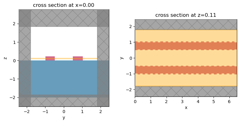
All the structures, sources, and monitors are consolidated, and the simulation is created and visualized.
[5]:
# list of all structures
structures = (
    [substrate, waveguide_1, waveguide_2]
    + corrug1_plus
    + corrug1_minus
    + corrug2_plus
    + corrug2_minus
)

# list of all sources
sources = [mode_src1, mode_src2]

# list of all monitors
monitors = [monitor_xy, monitor_flux_aligned, monitor_flux_misaligned]

# create the simulation
sim = td.Simulation(
    center=sim_center,
    size=sim_size,
    grid_spec=grid_spec,
    structures=structures,
    sources=sources,
    monitors=monitors,
    run_time=run_time,
    boundary_spec=boundary_spec,
)

# plot the simulation domain
f, (ax1, ax3) = plt.subplots(1, 2, tight_layout=True, figsize=(8, 4))
sim.plot(x=0, ax=ax1)
sim.plot(z=wg_height / 2, ax=ax3)
ax3.set_xlim(0, 20 * period)
plt.show()
Run Simulation#
[6]:
# run simulation
import tidy3d.web as web

sim_data = web.run(sim, task_name="bragg", path="data/bragg.hdf5", verbose=True)
19:24:24 CEST Created task 'bragg' with task_id
              'fdve-f05c0786-bfc2-485a-a9f1-c8ec30c5d38a' and task_type 'FDTD'.
              View task using web UI at
              'https://tidy3d.simulation.cloud/workbench?taskId=fdve-f05c0786-bf
              c2-485a-a9f1-c8ec30c5d38a'.
Task folder: 'default'.
19:24:26 CEST Maximum FlexCredit cost: 0.905. Minimum cost depends on task
              execution details. Use 'web.real_cost(task_id)' to get the billed
              FlexCredit cost after a simulation run.
19:24:27 CEST status = queued
              To cancel the simulation, use 'web.abort(task_id)' or
              'web.delete(task_id)' or abort/delete the task in the web UI.
              Terminating the Python script will not stop the job running on the
              cloud.
19:24:39 CEST status = preprocess
19:24:45 CEST starting up solver
19:24:46 CEST running solver
19:25:44 CEST early shutoff detected at 96%, exiting.
status = postprocess
19:25:46 CEST status = success
19:25:48 CEST View simulation result at
              'https://tidy3d.simulation.cloud/workbench?taskId=fdve-f05c0786-bf
              c2-485a-a9f1-c8ec30c5d38a'.
19:25:51 CEST loading simulation from data/bragg.hdf5
Field Plot#
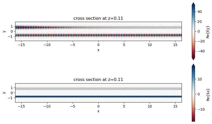
The frequency-domain fields are plotted in the xy plane cutting through the waveguides. We notice that the grating with aligned corrugation effectively reflects power at the design frequency, while the misalignment in the second grating causes it to be mostly transmissive.
[7]:
# plot fields on the monitor
fig, ax = plt.subplots(2, 1, tight_layout=True, figsize=(9, 5))
sim_data.plot_field(field_monitor_name="fields_xy", field_name="Ey", val="real", f=freq0, ax=ax[0])
sim_data.plot_field(field_monitor_name="fields_xy", field_name="Sx", val="real", f=freq0, ax=ax[1])
plt.show()
Transmission and Reflection#
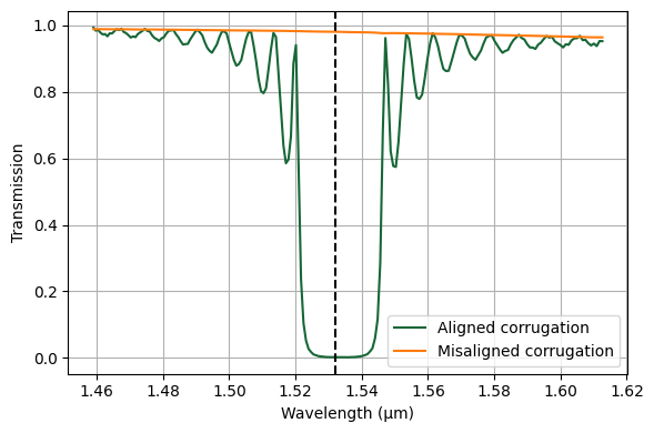
The observations made in the field plot above can be confirmed by plotting the flux recorded by the flux monitors as a function of frequency. In the region of the design frequency, indicated by the dashed black line, the drop in flux for the aligned-corrugation grating confirms its reflective property.
[8]:
fig, ax = plt.subplots(figsize=(6, 4), tight_layout=True)

# plot transmitted flux for each waveguide
ax.plot(td.C_0 / freqs, sim_data["flux_aligned"].flux, label="Aligned corrugation")
ax.plot(td.C_0 / freqs, sim_data["flux_misaligned"].flux, label="Misaligned corrugation")

# vertical line at design frequency
ax.axvline(td.C_0 / freq0, ls="--", color="k")

ax.set(xlabel="Wavelength (µm)", ylabel="Transmission")

ax.grid(True)
plt.legend()
plt.show()