Particle swarm optimization of a bullseye cavity for quantum emitter light extraction#
Note: the cost of running the entire notebook is higher than 10 FlexCredits.
A bullseye cavity is characterized by concentric rings of alternating dielectrics, resembling a bullseye target. It has been successfully employed to enhance the collection efficiency and decay rate of various quantum emitters, including quantum dots, defect centers in diamond, and 2D materials.
In this notebook, we show how to set up a bullseye cavity simulation using Tidy3D and use Particle Swarm Optimization (PSO) to enhance the coupling efficiency from quantum emitters into the fundamental mode of an optical fiber. We will use the Tidy3D Design plugin to manage the PSO (which uses the free available python library PySwarms) to easily create, compute and analyse the optimized bullseye cavity. For details about PSO you can
see the notebook Particle swarm optimization of a polarization beam splitter. In addition, we show how to calculate the cavity Purcell factor, which is another important figure-of-merit within the context of cavity electrodynamics.
Let’s start by importing the python libraries used throughout this notebook.
[1]:
# Uncomment the following line to install pyswarms if it's not installed in your environment already
# pip install pyswarms

# Standard python imports
import matplotlib.pylab as plt
import numpy as np

# Import regular tidy3d
import tidy3d as td
import tidy3d.plugins.design as tdd
import tidy3d.web as web
from tidy3d.plugins.mode import ModeSolver
from tidy3d.plugins.mode.web import run as run_mode_solver
Cavity Geometry and Simulation Parameters#
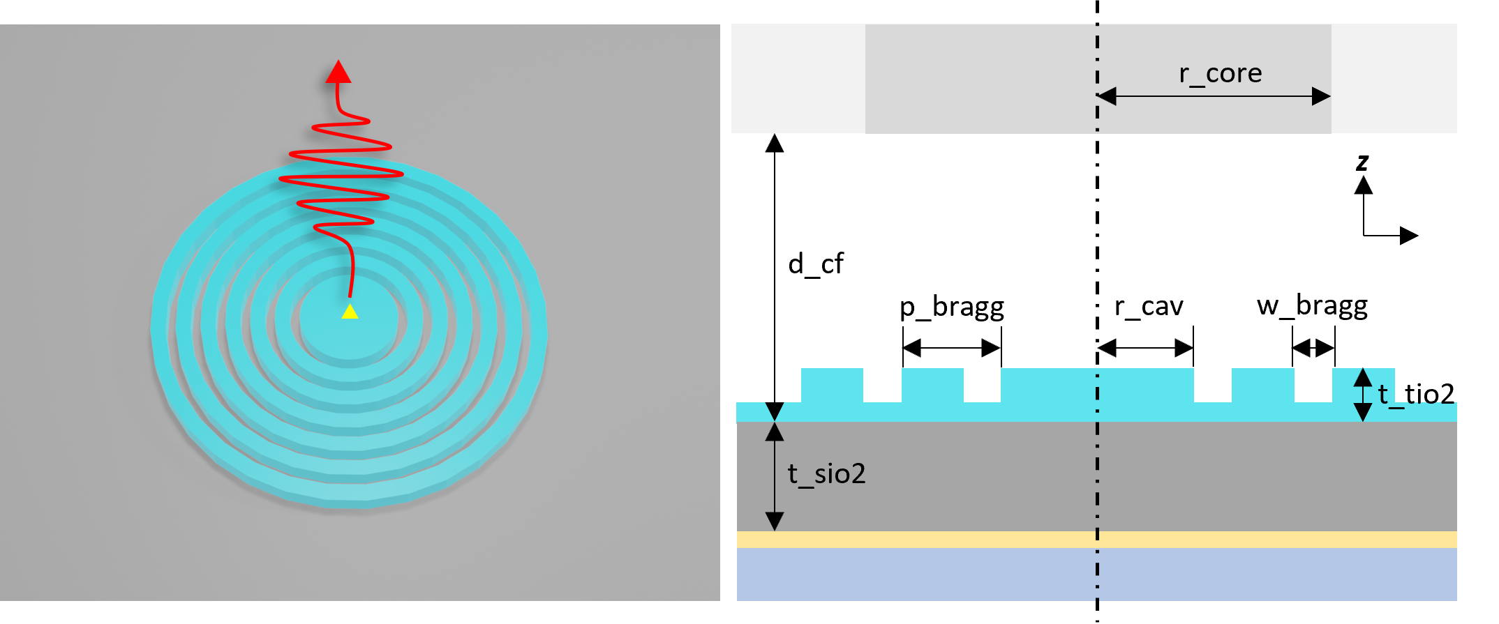
The cavity structure is inspired by Hekmati, R., Hadden, J.P., Mathew, A. et al. Bullseye dielectric cavities for photon collection from a surface-mounted quantum-light-emitter. Sci Rep 13, 5316 (2023) DOI: 10.1038/s41598-023-32359-0, where the authors presented a \(TiO_{2}\) over \(SiO_{2}\) bullseye cavity. In that work, the cavity was designed to enhance the emission from point sources, such as \(WSe_{2}\) flakes, single dye
molecules, and nano-diamonds, positioned just above the center of the structure. It was optimized using an iterative approach to enhance the power coupling into the numerical aperture (NA) of free-space optics and a low NA fiber.
Differently from that work, here we will set up the optimization to enhance the modal coupling efficiency of the generated photons into the collection fiber. When building an optimization scheme for practical applications, more advanced optimization strategies can be implemented to include other quantities of interest—for instance, the Purcell factor, which is important within the context of devices such as single-photon sources. The following figure shows the main cavity geometric parameters.
[2]:
# Initial parameters of the Bullseye cavity.
t_tio2 = 0.200  # TiO2 thin film thickness (um).
t_sio2 = 0.435  # SiO2 thin film thickness (um).
r_cav = 0.835  # Radius of the internal cavity (um).
p_bragg = 0.420  # Period of the Bragg reflector (um).
w_bragg = 0.155  # Gap width (etched region) of the Bragg reflector (um).
n_bragg = 8  # Number of Bragg periods.
n_tio2 = 2.50  # TiO2 refractive index (0.75 um).
n_sio2 = 1.45  # SiO2 refractive index (0.75 um).

# Collection fiber parameters (630HP).
r_core = 1.75  # Fiber core radius.
n_core = 1.46  # Core refractive index.
n_clad = 1.45  # Cladding refractive index.
d_cf = 2.0  # Distance between the cavity and the fiber.

# PSO optimization parameters.
iterations = 15  # Number of iterations.
n_particle = 5  # Number of particles in optimization.

# Simulation wavelength.
wl = 0.75  # Central simulation wavelength (um).
bw = 0.06  # Simulation bandwidth (um).
n_wl = 61  # Number of wavelength points within the bandwidth.
From the parameters defined before, a lot of variables are computed and used to set up the optimization.
[3]:
# Wavelengths and frequencies.
wl_max = wl + bw / 2
wl_min = wl - bw / 2
wl_range = np.linspace(wl_min, wl_max, n_wl)
freq = td.C_0 / wl
freqs = td.C_0 / wl_range
freqw = 0.5 * (freqs[0] - freqs[-1])
run_time = 5e-12  # Simulation run time.

# Material definition.
mat_tio2 = td.Medium(permittivity=n_tio2**2)  # TiO2 medium.
mat_sio2 = td.Medium(permittivity=n_sio2**2)  # SiO2 medium.
mat_etch = td.Medium(permittivity=1)  # Etch medium.
mat_core = td.Medium(permittivity=n_core**2)  # Fiber core medium.
mat_clad = td.Medium(permittivity=n_clad**2)  # Fiber cladding medium.

# Computational domain size.
pml_spacing = 0.6 * wl
eff_inf = 10
Bullseye Cavity Set Up#
We start with the definition of a function to build the bullseye cavity simulation. The PSO algorithm passes 6 parameters to this function, which in turn returns a simulation object. The quantum emitter is modeled as a y-oriented PointDipole placed at the top of the cavity surface. A ModeMonitor calculates the power coupled into the fiber fundamental mode, and a FluxMonitor gets the total dipole power. We are using a PECBoundary condition in the -z direction as a metallic
reflector at the bottom of the \(SiO_{2}\) layer.
[4]:
def get_simulation(
    r: float = r_cav,  # Cavity radius.
    p: float = p_bragg,  # Cavity period.
    w: float = w_bragg,  # Etched width.
    h: float = 0.0,  # Non-etched thickness with respect to TiO2 thickness.
    tsio2: float = t_sio2,  # SiO2 layer thickness.
    dcf: float = d_cf,  # Cavity to fiber distance.
) -> td.Simulation:
    """Create a Simulation of a bullseye cavity with variable geometry and material thickness."""

    # Computational domain size.
    size_x = 2 * pml_spacing + max(2 * (r + n_bragg * p), 2 * r_core)
    size_y = size_x
    size_z = pml_spacing + tsio2 + t_tio2 + dcf
    center_z = -size_z / 2
    qd_pos_z = tsio2 + t_tio2
    mon_pos_z = size_z - pml_spacing / 2

    # Point dipole source located at the center of TiO2 thin film.
    dp_source = td.PointDipole(
        center=(0, 0, qd_pos_z),
        source_time=td.GaussianPulse(freq0=freq, fwidth=freqw),
        polarization="Ey",
    )

    # Field monitor to visualize the fields in xy plane.
    field_monitor_xy = td.FieldMonitor(
        center=(0, 0, qd_pos_z - t_tio2 / 2),
        size=(size_x, size_y, 0),
        freqs=[freq],
        name="field_xy",
    )

    # Field monitor to visualize the fields in xz plane.
    field_monitor_xz = td.FieldMonitor(
        center=(0, 0.05, size_z / 2),
        size=(size_x, 0, size_z),
        freqs=[freq],
        name="field_xz",
    )

    # Mode monitor to get the power coupled into the fiber modes.
    mode_spec = td.ModeSpec(num_modes=1, target_neff=n_core)
    mode_monitor = td.ModeMonitor(
        center=(0, 0, mon_pos_z),
        size=(size_x, size_y, 0),
        freqs=freqs,
        mode_spec=mode_spec,
        name="mode_fiber",
    )

    # Flux monitor to get the total dipole power.
    flux_dip = td.FluxMonitor(
        center=(0, 0, size_z / 2),
        size=(0.8 * size_x, 0.8 * size_y, size_z),
        freqs=freqs,
        exclude_surfaces=("z-",),
        name="flux_dip",
    )

    # Silicon dioxide layer
    sio2_layer = td.Structure(
        geometry=td.Box.from_bounds(
            rmin=(-size_x / 2 - eff_inf, -size_y / 2 - eff_inf, -eff_inf),
            rmax=(size_x / 2 + eff_inf, size_y / 2 + eff_inf, tsio2),
        ),
        medium=mat_sio2,
    )

    # Fiber cladding
    fiber_clad = td.Structure(
        geometry=td.Box.from_bounds(
            rmin=(-size_x / 2 - eff_inf, -size_y / 2 - eff_inf, size_z - pml_spacing),
            rmax=(size_x / 2 + eff_inf, size_y / 2 + eff_inf, size_z + eff_inf),
        ),
        medium=mat_clad,
    )

    # Fiber core
    fiber_core = td.Structure(
        geometry=td.Cylinder(
            radius=r_core,
            center=(0, 0, size_z + (((pml_spacing + eff_inf) / 2) - pml_spacing)),
            axis=2,
            length=pml_spacing + eff_inf,
        ),
        medium=mat_core,
    )

    # Bullseye cavity
    bullseye = []
    cyl_rad = n_bragg * p + r
    for _ in range(0, n_bragg):
        bullseye.append(
            td.Structure(
                geometry=td.Cylinder(
                    radius=cyl_rad,
                    center=(0, 0, qd_pos_z - t_tio2 / 2),
                    axis=2,
                    length=t_tio2,
                ),
                medium=mat_tio2,
            )
        )
        bullseye.append(
            td.Structure(
                geometry=td.Cylinder(
                    radius=cyl_rad - p + w,
                    center=(0, 0, qd_pos_z - t_tio2 / 2),
                    axis=2,
                    length=t_tio2,
                ),
                medium=mat_etch,
            )
        )
        cyl_rad -= p

    bullseye.append(
        td.Structure(
            geometry=td.Cylinder(
                radius=r, center=(0, 0, qd_pos_z - t_tio2 / 2), axis=2, length=t_tio2
            ),
            medium=mat_tio2,
        )
    )
    # Non-etched TiO2 region.
    if h > 0:
        bullseye.append(
            td.Structure(
                geometry=td.Box.from_bounds(
                    rmin=(-size_x / 2 - eff_inf, -size_y / 2 - eff_inf, tsio2),
                    rmax=(
                        size_x / 2 + eff_inf,
                        size_y / 2 + eff_inf,
                        tsio2 + h * t_tio2,
                    ),
                ),
                medium=mat_tio2,
            )
        )

    # Simulation definition
    sim = td.Simulation(
        center=(0, 0, -center_z),
        size=(size_x, size_y, size_z),
        medium=mat_etch,
        grid_spec=td.GridSpec.auto(min_steps_per_wvl=15, wavelength=wl),
        structures=[sio2_layer, fiber_clad, fiber_core] + bullseye,
        sources=[dp_source],
        normalize_index=0,
        monitors=[field_monitor_xy, field_monitor_xz, mode_monitor, flux_dip],
        boundary_spec=td.BoundarySpec(
            x=td.Boundary.pml(),
            y=td.Boundary.pml(),
            z=td.Boundary(minus=td.PECBoundary(), plus=td.PML()),
        ),
        symmetry=(1, -1, 0),
        run_time=run_time,
    )
    return sim
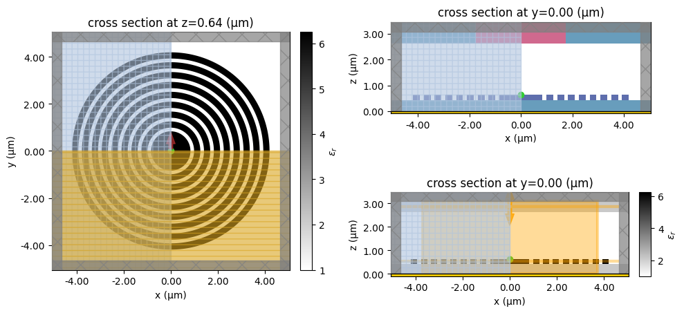
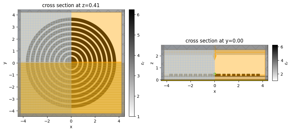
Let’s visualize the simulation set up and verify if all the elements are in their correct places.
[5]:
init_design = get_simulation()

fig = plt.figure(tight_layout=True, figsize=(10, 5))
gs = fig.add_gridspec(2, 2)
ax1 = fig.add_subplot(gs[:, 0])
ax2 = fig.add_subplot(gs[0, 1])
ax3 = fig.add_subplot(gs[1, 1])
init_design.plot_eps(z=t_sio2 + t_tio2, ax=ax1, monitor_alpha=0)
init_design.plot(y=0, ax=ax2, monitor_alpha=0)
init_design.plot_eps(y=0, ax=ax3)
plt.show()
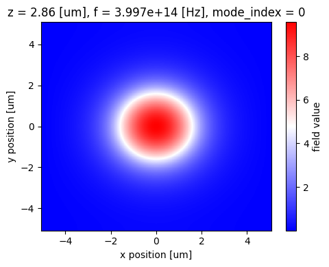
Output Fiber Mode#
Before running the optimization, we will make sure the correct optical fiber mode has been considered.
[6]:
mode_spec = td.ModeSpec(num_modes=1, target_neff=n_core)
mode_solver = ModeSolver(
    simulation=init_design,
    plane=td.Box(
        center=(0, 0, 0.5 * pml_spacing + t_sio2 + t_tio2 + d_cf),
        size=(td.inf, td.inf, 0),
    ),
    mode_spec=mode_spec,
    freqs=[freq],
)
mode_fiber = run_mode_solver(mode_solver)
19:24:36 CEST WARNING: Mode monitor 'mode_fiber' has a large number (2.18e+05)
              of grid points. This can lead to solver slow-down and increased
              cost. Consider making the size of the component smaller, as long
              as the modes of interest decay by the plane boundaries.
19:24:37 CEST Mode solver created with
              task_id='fdve-48610c46-ccd6-42d4-8853-6ba946535ab2',
              solver_id='mo-92a61d5d-c640-4231-94c3-5e326bae02a5'.
19:24:40 CEST Mode solver status: queued
19:24:42 CEST Mode solver status: running
19:25:05 CEST Mode solver status: success
We can see the y-oriented fundamental optical fiber mode, as desired.
[7]:
fig, ax = plt.subplots(1, 1, figsize=(5, 4), tight_layout=True)
mode_fiber.Ey.real.sel(mode_index=0, f=freq).plot(x="x", y="y", cmap="bwr", ax=ax)
plt.show()
Particle Swarm Optimization#
The figure-of-merit used in the optimization is the coupling efficiency of generated photons into the fundamental optical mode of the collection fiber. We need to normalize the modal power by the dipole power to obtain the correct value, as below.
[8]:
# Figure of Merit (FOM) calculation.
def get_coupling_eff(sim_data: td.SimulationData) -> float:
    """Return the power at the mode index of interest."""
    mode_amps = sim_data["mode_fiber"].amps.sel(direction="+", mode_index=0)
    mode_power = np.squeeze(np.abs(mode_amps) ** 2)
    dip_power = sim_data["flux_dip"].flux
    return mode_power / dip_power
Now we can define the pre and post functions that the DesignSpace needs to carry out the PSO. The fn_pre will receive keyword arguments suggested from the optimizer and returns a Simulation object. This Simulation will automatically be combined into a Batch and run in parallel on the Tidy3D cloud, for fast computation of each PSO iteration.
The fn_post function receives the SimulationData from the computation and calculates the maximising FOM defined above. All optimizers in the Design plugin are maximising functions so no minus sign is needed to reverse this FOM. The output float value is fed to the PSO to evaluate the current solution and improve the next suggestion.
[9]:
def fn_pre(r: float, p: float, w: float, h: float, t_sio2: float, dcf: float) -> td.Simulation:
    """Build a Simulation object from parameters suggested by the PSO."""
    sim = get_simulation(r, p, w, h, t_sio2, dcf)
    return sim


def fn_post(sim_data: td.SimulationData) -> float:
    """Analyze SimulationData from a bullseye cavity simulation and return coupling efficiency."""
    ce = np.max(get_coupling_eff(sim_data))
    return float(ce)
Each parameter is then defined with the name matching the argument in fn_pre. The PSO will work within the bounds specified in the span to suggest solutions. To make this notebook reproducible we also define the initial position and set the seed - though this isn’t necessary for every PSO run.
In the Method we define the hyperparameters used to setup the PSO (the inertia weight, the cognitive coefficient, and the social coefficient) which typically require some experimentation to find the optimum values. We have done some iteration to choose these values, but they could likely be refined further.
The Method and Parameters are then input to the DesignSpace which controls the optimization and returns the results.
[10]:
# Setup parameters for DesignSpace
r_param = tdd.ParameterFloat(name="r", span=(0.5 * r_cav, 1.5 * r_cav))
p_param = tdd.ParameterFloat(name="p", span=(0.5 * p_bragg, 1.5 * p_bragg))
w_param = tdd.ParameterFloat(name="w", span=(0.5 * w_bragg, 1.5 * w_bragg))
h_param = tdd.ParameterFloat(name="h", span=(0.0, 1.0))
t_sio2_param = tdd.ParameterFloat(name="t_sio2", span=(0.5 * t_sio2, 1.5 * t_sio2))
dcf_param = tdd.ParameterFloat(name="dcf", span=(0.5 * d_cf, 1.5 * d_cf))
parameters = (r_param, p_param, w_param, h_param, t_sio2_param, dcf_param)

# Initial parameters
np.random.seed(3)
init_par = np.random.uniform(0.5, 1.0, (n_particle, len(parameters)))
init_par[:, 0] = init_par[:, 0] * r_cav
init_par[:, 1] = init_par[:, 1] * p_bragg
init_par[:, 2] = init_par[:, 2] * w_bragg
init_par[:, 3] = init_par[:, 3] - 0.5
init_par[:, 4] = init_par[:, 4] * t_sio2
init_par[:, 5] = init_par[:, 5] * d_cf

particle_swarm = tdd.MethodParticleSwarm(
    n_particles=n_particle,
    n_iter=iterations,
    cognitive_coeff=0.5,
    social_coeff=0.3,
    weight=0.9,
    init_pos=init_par,
)

design_space = tdd.DesignSpace(
    method=particle_swarm, parameters=parameters, task_name="PSO_Notebook", path_dir="./data"
)
Now, we are ready to run the optimization!
[11]:
td.config.logging.level = "ERROR"

# Run the optimization
results = design_space.run(fn_pre, fn_post, verbose=True)
df = results.to_dataframe()
2025-07-27 19:25:08,416 - pyswarms.single.global_best - INFO - Optimize for 15 iters with {'c1': 0.5, 'c2': 0.3, 'w': 0.9}
pyswarms.single.global_best:   0%|          |0/15
19:25:08 CEST Running 5 Simulations
pyswarms.single.global_best: 7%|▋ |1/15, best_cost=-0.114
19:30:24 CEST Running 5 Simulations
pyswarms.single.global_best: 13%|█▎ |2/15, best_cost=-0.154
19:52:43 CEST Running 5 Simulations
pyswarms.single.global_best: 20%|██ |3/15, best_cost=-0.227
19:57:15 CEST Running 5 Simulations
pyswarms.single.global_best: 27%|██▋ |4/15, best_cost=-0.227
19:59:48 CEST Running 5 Simulations
pyswarms.single.global_best: 33%|███▎ |5/15, best_cost=-0.227
20:01:54 CEST Running 5 Simulations
pyswarms.single.global_best: 40%|████ |6/15, best_cost=-0.227
20:17:59 CEST Running 5 Simulations
pyswarms.single.global_best: 47%|████▋ |7/15, best_cost=-0.227
20:33:52 CEST Running 5 Simulations
pyswarms.single.global_best: 53%|█████▎ |8/15, best_cost=-0.227
20:42:44 CEST Running 5 Simulations
pyswarms.single.global_best: 60%|██████ |9/15, best_cost=-0.332
20:48:51 CEST Running 5 Simulations
pyswarms.single.global_best: 67%|██████▋ |10/15, best_cost=-0.332
20:55:28 CEST Running 5 Simulations
pyswarms.single.global_best: 73%|███████▎ |11/15, best_cost=-0.332
21:00:12 CEST Running 5 Simulations
pyswarms.single.global_best: 80%|████████ |12/15, best_cost=-0.332
21:06:12 CEST Running 5 Simulations
pyswarms.single.global_best: 87%|████████▋ |13/15, best_cost=-0.332
21:11:12 CEST Running 5 Simulations
pyswarms.single.global_best: 93%|█████████▎|14/15, best_cost=-0.332
21:17:22 CEST Running 5 Simulations
pyswarms.single.global_best: 100%|██████████|15/15, best_cost=-0.332
2025-07-27 21:23:00,664 - pyswarms.single.global_best - INFO - Optimization finished | best cost: -0.3316597424081307, best pos: [0.74632414 0.3812908  0.12455691 0.26602631 0.64924378 1.0869887 ]
21:23:00 CEST Best Result: -0.3316597424081307
              Best Parameters: r: 0.7463241440689826 p: 0.3812907960183133 w:
              0.1245569125769858 h: 0.26602630907617625 t_sio2:
              0.6492437787750074 dcf: 1.0869886995014149
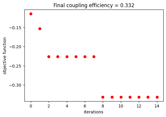
Ultimately, we can obtain the optimized cavity parameters and see how the optimization has evolved into the final value. When optimizing a device for practical applications, one can consider adding more particles, increasing the number of iterations, or trying different metaparameters to improve results.
[12]:
# The optimizer object is stored in the results from the DesignSpace
best_par = results.optimizer.swarm.best_pos
cost_history = results.optimizer.cost_history

print("Best parameters:")
print(f"r_cav = {best_par[0]:.3f} um")
print(f"p_bragg = {best_par[1]:.3f} um")
print(f"w_bragg = {best_par[2]:.3f} um")
print(f"h = {best_par[3]:.3f}")
print(f"t_sio2 = {best_par[4]:.3f} um")
print(f"d_cf = {best_par[5]:.3f} um")

fig, ax = plt.subplots(1, 1, figsize=(6, 4))
ax.plot(cost_history, "ro")
ax.set_xlabel("iterations")
ax.set_ylabel("objective function")
ax.set_title(f"Final coupling efficiency = {-min(cost_history):.3f}")
plt.show()
Best parameters:
r_cav = 0.746 um
p_bragg = 0.381 um
w_bragg = 0.125 um
h = 0.266
t_sio2 = 0.649 um
d_cf = 1.087 um
Final Bullseye Cavity#
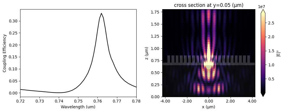
Now, we can simulate the optimized bullseye cavity and take a look at the coupling efficiency along the whole bandwidth.
[13]:
final_design = get_simulation(
    r=best_par[0],
    p=best_par[1],
    w=best_par[2],
    h=best_par[3],
    tsio2=best_par[4],
    dcf=best_par[5],
)

# Field monitor to visualize the fields at the peak coupling efficiency.
wl_mon = 0.725  # Wavelength for field monitor.
field_monitor_xz_f = td.FieldMonitor(
    center=(0, 0.05, final_design.center[2] / 2),
    size=(final_design.size[0], 0, final_design.size[2]),
    freqs=[td.C_0 / wl_mon],
    name="field_xz_f",
)

mon_f = final_design.monitors + (field_monitor_xz_f,)
final_design = final_design.copy(update=dict(monitors=mon_f))

fig, (ax1, ax2) = plt.subplots(1, 2, tight_layout=True, figsize=(10, 5))
final_design.plot_eps(z=best_par[4] + t_tio2 / 1.5, ax=ax1)
final_design.plot_eps(y=0, ax=ax2)
plt.show()
[14]:
sim_data_final = web.run(final_design, task_name="final bullseye")
21:23:01 CEST Created task 'final bullseye' with task_id
              'fdve-99af72a9-aba1-4e1e-80b5-964f4cdf6b19' and task_type 'FDTD'.
              View task using web UI at
              'https://tidy3d.simulation.cloud/workbench?taskId=fdve-99af72a9-ab
              a1-4e1e-80b5-964f4cdf6b19'.
Task folder: 'default'.
21:23:03 CEST Maximum FlexCredit cost: 0.329. Minimum cost depends on task
              execution details. Use 'web.real_cost(task_id)' to get the billed
              FlexCredit cost after a simulation run.
21:23:04 CEST status = queued
              To cancel the simulation, use 'web.abort(task_id)' or
              'web.delete(task_id)' or abort/delete the task in the web UI.
              Terminating the Python script will not stop the job running on the
              cloud.
21:23:55 CEST starting up solver
running solver
21:24:22 CEST early shutoff detected at 20%, exiting.
status = postprocess
21:24:46 CEST status = success
21:24:48 CEST View simulation result at
              'https://tidy3d.simulation.cloud/workbench?taskId=fdve-99af72a9-ab
              a1-4e1e-80b5-964f4cdf6b19'.
21:24:51 CEST loading simulation from simulation_data.hdf5
The peak coupling efficiency is about 33% at 0.76 \(\mu m\).
[15]:
coup_eff = get_coupling_eff(sim_data_final)

f, (ax1, ax2) = plt.subplots(1, 2, figsize=(10, 4), tight_layout=True)
ax1.plot(wl_range, coup_eff, "-k")
ax1.set_xlabel("Wavelength (um)")
ax1.set_ylabel("Coupling Efficiency")
ax1.set_xlim(wl - bw / 2, wl + bw / 2)
sim_data_final.plot_field("field_xz_f", "E", "abs^2", ax=ax2)
ax2.set_aspect("auto")
plt.show()
Purcell Factor Calculation#
Purcell factor enhancement is usually desired when designing a quantum emitter light extractor device, as it can lead to higher photon generation rates, \(\beta\)-factors, and photon indistinguishability. Next, we calculate the bullseye nanocavity Purcell factor (\(F_{p} = P_{cav}/P_{bulk}\)) defined as the ratio between the dipole power emitted in final device and in the bulk semiconductor.
We can calculate \(P_{bulk}\) analytically as
\(P_{bulk_a} = \frac{\omega^{2}}{12\pi}\frac{\mu_{0}n}{c}\)
where \(n\) is the refractive index of the quantum emitter host material.
[16]:
p_bulk_a = ((2 * np.pi * freqs) ** 2 / (12 * np.pi)) * (td.MU_0 * n_tio2 / td.C_0)
When symmetries are present in the simulation, dipole image charges are included for each symmetry plane due to field continuity reasons. In this case, we need to adjust \(P_{bulk_a}\) as below:
[17]:
p_bulk_a = p_bulk_a * 2 ** (2 * np.sum(np.abs(final_design.symmetry)))
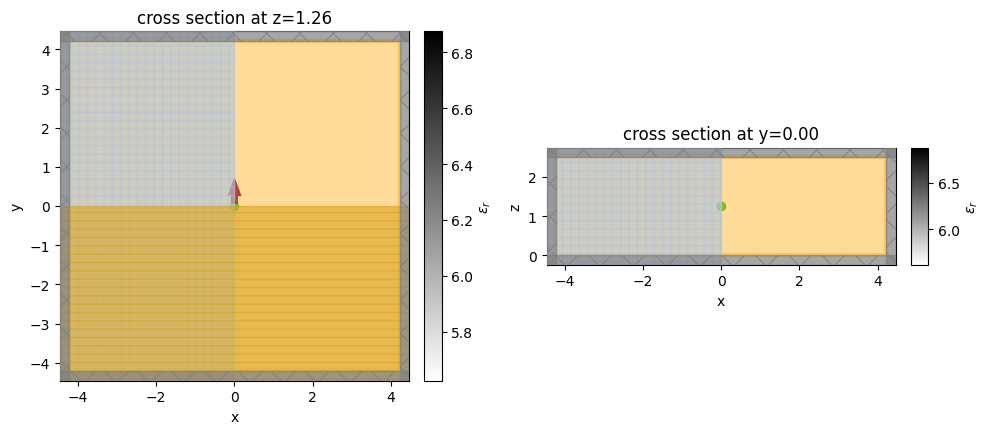
Another way of obtaining \(P_{bulk}\) is through a normalization run considering the quantum emitter embedded in a homogeneous medium, as follows. Note that the same symmetry condition of the cavity simulation should be used.
[18]:
# Point dipole source located at the center of TiO2 thin film.
dp_source_bulk = td.PointDipole(
    center=(0, 0, final_design.size[2] / 2),
    source_time=td.GaussianPulse(freq0=freq, fwidth=freqw),
    polarization="Ey",
)

# Flux monitor to get the total dipole power.
flux_dip_bulk = td.FluxMonitor(
    center=(0, 0, final_design.size[2] / 2),
    size=final_design.size,
    freqs=freqs,
    name="flux_dip_bulk",
)

bulk_device = final_design.copy(
    update={
        "structures": [],
        "sources": [dp_source_bulk],
        "monitors": [flux_dip_bulk],
        "medium": mat_tio2,
        "symmetry": final_design.symmetry,
        "boundary_spec": td.BoundarySpec.all_sides(boundary=td.PML()),
    }
)

fig, (ax1, ax2) = plt.subplots(1, 2, tight_layout=True, figsize=(10, 5))
bulk_device.plot_eps(z=(final_design.size[2]) / 2, ax=ax1)
bulk_device.plot_eps(y=0, ax=ax2)
plt.show()
[19]:
sim_data_bulk = web.run(bulk_device, task_name="bulk sim")
21:24:52 CEST Created task 'bulk sim' with task_id
              'fdve-cc33508a-b7b4-45d8-a494-a1911905f86d' and task_type 'FDTD'.
              View task using web UI at
              'https://tidy3d.simulation.cloud/workbench?taskId=fdve-cc33508a-b7
              b4-45d8-a494-a1911905f86d'.
Task folder: 'default'.
21:24:54 CEST Maximum FlexCredit cost: 0.362. Minimum cost depends on task
              execution details. Use 'web.real_cost(task_id)' to get the billed
              FlexCredit cost after a simulation run.
21:24:55 CEST status = queued
              To cancel the simulation, use 'web.abort(task_id)' or
              'web.delete(task_id)' or abort/delete the task in the web UI.
              Terminating the Python script will not stop the job running on the
              cloud.
21:25:22 CEST status = preprocess
21:25:26 CEST starting up solver
21:25:27 CEST running solver
21:25:30 CEST early shutoff detected at 4%, exiting.
status = success
              View simulation result at
              'https://tidy3d.simulation.cloud/workbench?taskId=fdve-cc33508a-b7
              b4-45d8-a494-a1911905f86d'.
21:25:32 CEST loading simulation from simulation_data.hdf5
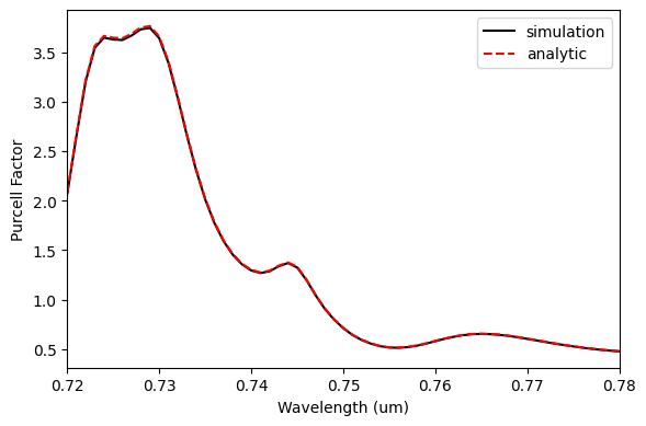
A maximum Purcell value of about 4.75 is achieved at 0.76 \(\mu m\), even though this figure-of-merit was not pursued along the optimization. Higher Purcell values can be obtained in cases where the quantum emitter can be embedded within the cavity material.
[20]:
p_cav = sim_data_final["flux_dip"].flux
p_bulk_s = sim_data_bulk["flux_dip_bulk"].flux

purcell_s = p_cav / p_bulk_s
purcell_a = p_cav / p_bulk_a

f, ax1 = plt.subplots(1, 1, figsize=(6, 4), tight_layout=True)
ax1.plot(wl_range, purcell_s, "-k", label="simulation")
ax1.plot(wl_range, purcell_a, "--r", label="analytic")
ax1.set_xlabel("Wavelength (um)")
ax1.set_ylabel("Purcell Factor")
ax1.set_xlim(wl - bw / 2, wl + bw / 2)
plt.legend()
plt.show()