Adjoint optimization of a wavelength division multiplexer#
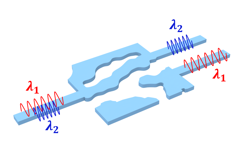
In this notebook, we will use a multi-objective optimization to design a wavelength division multiplexer (WDM).
In short, this device takes in broadband light and directs light of different wavelengths to different output ports.
This demo combines the basic setup of our 3rd tutorial of a mode converter with the multi-frequency feature introduced in Tidy3D version 2.5.
We will follow many of the parameters outlined in Cheung, Alfred KC, et al. "Inverse-designed CWDM demultiplexer operated in O-band." Optical Fiber Communication Conference. Optica Publishing Group, 2024. Although, to reduce the flex credit usage and run time, our setup will use a smaller device, run using a 2D simulation, and use a lower resolution.
If you are unfamiliar with inverse design, we also recommend our intro to inverse design tutorials and our primer on automatic differentiation with tidy3d.
[1]:
import autograd as ag
import autograd.numpy as anp
import matplotlib.pylab as plt
import numpy as np
import tidy3d as td
import tidy3d.web as web
Setup#
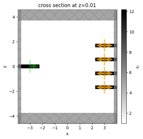
First we set up our basic simulation.
We have an input waveguide connected to a square design region, which has n=4 output waveguides.
The square design region is a custom medium with a pixelated permittivity grid that we wish to optimize such that input light of different wavelengths get directed to different output ports.
As this is a SOI device, we typically define the design region and waveguides as Silicon sitting on an SiO2 substrate. For this demo, we make a 2D simulation, but it can be easily made 3D by changing the Lz parameter, adding dimension to the structures, and adding a substrate.
[2]:
# material information
n_si = 3.49
n_sio2 = 1.45  # not used in 2D
n_air = 1

# channel wavelengths
wvls_design = np.array([1.270, 1.290, 1.310, 1.330])

freqs_design = td.C_0 / wvls_design
num_freqs_design = len(freqs_design)
freq_max = np.max(freqs_design)
freq_min = np.min(freqs_design)
keys = [str(i) for i in range(num_freqs_design)]
df_design = abs(np.mean(np.diff(freqs_design)))

# forward source
freq0 = np.mean(freqs_design)
wvl0 = td.C_0 / freq0
fwidth = freq_max - freq_min
run_time = 200 / fwidth

# we average the metrics over the channels with some frequency width
channel_fwidth = df_design / 2.0
channel_bounds = [(f - channel_fwidth / 2, f + channel_fwidth / 2) for f in freqs_design]
num_freqs_channel = 5
channel_freqs = []
for fmin, fmax in channel_bounds:
    sub_freqs = np.linspace(fmin, fmax, num_freqs_channel)
    channel_freqs += sub_freqs.tolist()

# size of design region
lx = 4.5
ly = 4.5
ly_single = ly / num_freqs_design
lz = td.inf

# size of waveguides
wg_width = 0.3
wg_length = 1.5
wg_spacing = 0.8

# spacing between design region and PML in y
buffer = 1.5

# size of simulation
Lx = lx + wg_length * 2
Ly = ly + buffer * 2
Lz = 0.0

# fabrication constraints (feature size and projection strength)
radius = 0.100
beta0 = 2

# resolution information
min_steps_per_wvl = 18
dl_design_region = 0.015
Static Simulation#
First, we’ll define the simulation without any design region using the “static” components that don’t change over the optimization.
[3]:
# define the waveguide ports
wg_in = td.Structure(
    geometry=td.Box(
        center=(-Lx / 2, 0, 0),
        size=(wg_length * 2, wg_width, lz),
    ),
    medium=td.Medium(permittivity=n_si**2),
)

centers_y = np.linspace(-ly / 2.0 + ly_single / 2.0, +ly / 2.0 - ly_single / 2.0, num_freqs_design)
mode_size = (0, 0.9 * ly_single, td.inf)

wgs_out = []
for center_y in centers_y:
    wg_out = td.Structure(
        geometry=td.Box(
            center=(+Lx / 2, center_y, 0),
            size=(wg_length * 2, wg_width, lz),
        ),
        medium=td.Medium(permittivity=n_si**2),
    )
    wgs_out.append(wg_out)

# measure the mode amplitudes at each of the output ports
mnts_mode = []
for key, center_y in zip(keys, centers_y):
    mnt_mode = td.ModeMonitor(
        center=(Lx / 2 - wg_length / 2, center_y, 0),
        size=mode_size,
        freqs=channel_freqs,
        mode_spec=td.ModeSpec(),
        name=f"mode_{key}",
    )
    mnts_mode.append(mnt_mode)

# measures the flux at each of the output ports
mnts_flux = []
for key, center_y in zip(keys, centers_y):
    mnt_flux = td.FluxMonitor(
        center=(Lx / 2 - wg_length / 2, center_y, 0),
        size=mode_size,
        freqs=channel_freqs,
        name=f"flux_{key}",
    )
    mnts_flux.append(mnt_flux)

# and a field monitor that measures fields on the z=0 plane at the design freqs
fld_mnt = td.FieldMonitor(
    center=(0, 0, 0),
    size=(td.inf, td.inf, 0),
    freqs=freqs_design,
    name="field",
)

# inject the fundamental mode into the input waveguide
mode_src = td.ModeSource(
    center=(-Lx / 2 + wg_length / 2, 0, 0),
    size=mode_size,
    source_time=td.GaussianPulse(
        freq0=freq0,
        fwidth=fwidth,
    ),
    direction="+",
    mode_index=0,
)

sim_static = td.Simulation(
    size=(Lx, Ly, Lz),
    grid_spec=td.GridSpec.auto(
        min_steps_per_wvl=min_steps_per_wvl,
        wavelength=np.min(wvls_design),
    ),
    structures=[wg_in] + wgs_out,
    sources=[mode_src],
    monitors=mnts_mode + mnts_flux + [fld_mnt],
    boundary_spec=td.BoundarySpec.pml(x=True, y=True, z=True if Lz else False),
    run_time=run_time,
)
[4]:
ax = sim_static.plot_eps(z=0.01)
ax.set_aspect("equal")
Solving modes#
Next, we want to ensure that we are injecting and measuring the right waveguide modes at each of the ports.
We’ll use tidy3d’s ModeSolver to analyze the modes of our input waveguide.
[5]:
from tidy3d.plugins.mode import ModeSolver
from tidy3d.plugins.mode.web import run as run_mode_solver

# we'll ask for 4 modes just to inspect
num_modes = 4

# let's define how large the mode planes are and how far they are from the PML relative to the design region
mode_size = (0, ly_single, td.inf)

# make a plane corresponding to where we wish to measure the input mode
plane_in = td.Box(
    center=(-Lx / 2 + wg_length / 2.0, 0, 0),
    size=mode_size,
)

mode_solver = ModeSolver(
    simulation=sim_static,
    plane=plane_in,
    freqs=freqs_design,
    mode_spec=td.ModeSpec(num_modes=num_modes),
)
Next we run the mode solver on the servers.
[6]:
mode_data = run_mode_solver(mode_solver, reduce_simulation=True)
14:06:30 CET Mode solver created with
             task_id='fdve-4ed6c7c9-1a96-4641-8dbc-9c6cb1e0b0ca',
             solver_id='mo-2c8da480-9927-4c0a-9153-1bf1a78a1c08'.
14:06:34 CET Mode solver status: queued
14:07:05 CET Mode solver status: running
14:07:10 CET Mode solver status: success
And visualize the results.
[7]:
fig, axs = plt.subplots(num_modes, 3, figsize=(12, 12), tight_layout=True)
for mode_index in range(num_modes):
    vmax = 1.1 * max(
        abs(mode_data.field_components[n].sel(mode_index=mode_index)).max()
        for n in ("Ex", "Ey", "Ez")
    )
    for field_name, ax in zip(("Ex", "Ey", "Ez"), axs[mode_index]):
        for freq in freqs_design:
            key = f"{td.C_0 / freq * 1000:.0f} nm"
            field = mode_data.field_components[field_name].sel(mode_index=mode_index, f=freq)
            field.real.plot(label=f"Real ({key})", ax=ax)
            field.imag.plot(ls="--", label=f"Imag ({key})", ax=ax)
        ax.set_title(f"index={mode_index}, {field_name}")
        ax.set_ylim(-vmax, vmax)
        ax.legend()

print("Effective index of computed modes: ", np.array(mode_data.n_eff))
Effective index of computed modes:  [[3.15138964 2.84079307 2.00642254 1.09893523]
 [3.14368787 2.81919688 1.9704335  1.09132187]
 [3.13596834 2.79719528 1.93431963 1.08470219]
 [3.1282325  2.77478564 1.89808873 1.07888052]]
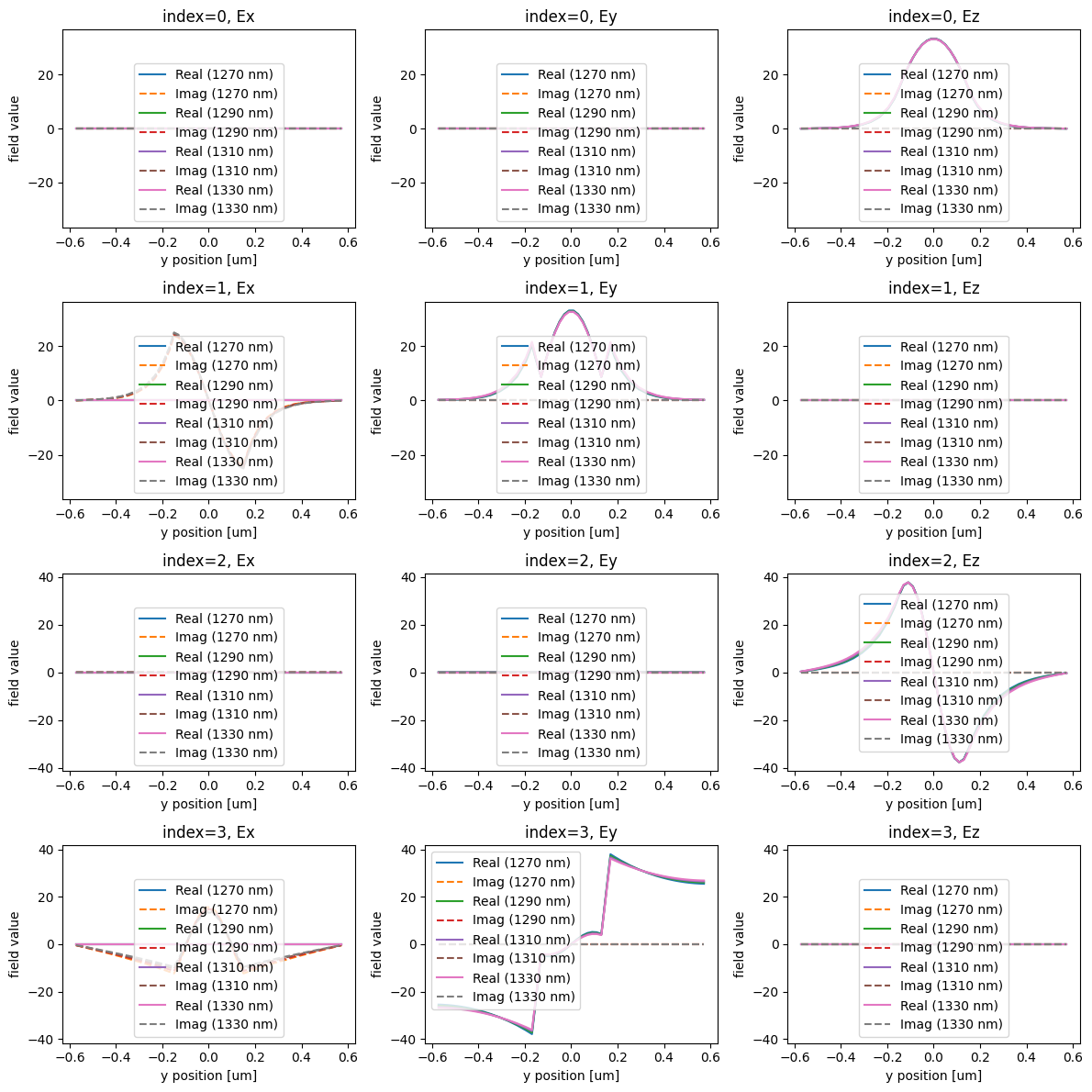
We identify mode_index=0 as the first order mode that is out of plane of the device. Let’s choose to optimize our device with respect to this as the mode of interest for both the input and output.
We’ll update or static simulation with the new mode index and mode specification, in case these are different from the original ones.
[8]:
mode_index = 0
mode_spec = td.ModeSpec(num_modes=mode_index + 1)

sim_static = sim_static.updated_copy(mode_index=mode_index, path="sources/0")
sim_static = sim_static.updated_copy(mode_spec=mode_spec, path="sources/0")
for i in range(num_freqs_design):
    sim_static = sim_static.updated_copy(mode_spec=mode_spec, path=f"monitors/{i}")
Define design region#
Next, we define the design region as a pixelated grid of permittivity values that get generated from our optimization parameters.
We first define the overall geometry as a td.Box and also the number of pixels in x and y based on our design region resolution.
[9]:
nx = int(lx / dl_design_region)
ny = int(ly / dl_design_region)

design_region_geo = td.Box(size=(lx, ly, lz), center=(0, 0, 0))
Next we write a function to give us the pixelated array as a function of our parameters through our filtering and projection methods, which are used to make the resulting structures easier to fabricate. For more details, refer to our 4th lecture in the inverse design 101 lecture series, which focuses on fabrication constraints.
We also wrap this function in another one that generates the entire td.Structure corresponding to the design region, for convenience later.
[10]:
from tidy3d.plugins.autograd import make_filter_and_project, rescale

filter_project = make_filter_and_project(radius, dl_design_region)


def get_density(params: np.ndarray, beta: float) -> np.ndarray:
    """Get the density of material (0, 1) as a function of the parameters (0,1)"""
    return filter_project(params, beta=beta)


def make_eps(params: np.ndarray, beta: float) -> np.ndarray:
    """Construct density values and rescale them to relative permittivity values between air and silicon."""
    density = get_density(params, beta=beta)
    return rescale(density, 1, n_si**2)


def make_custom_medium(params: np.ndarray, beta: float) -> td.Structure:
    """Make td.Structure containing custom medium with the permittivity data as a function of parameters."""
    eps = make_eps(params, beta).reshape((nx, ny, 1))
    xs = anp.linspace(-lx / 2, lx / 2, nx)
    ys = anp.linspace(-ly / 2, ly / 2, ny)
    zs = [0]
    coords = dict(x=xs, y=ys, z=zs)

    eps_arr = td.ScalarFieldDataArray(data=eps, coords=coords)

    medium = td.CustomMedium(permittivity=eps_arr)

    return td.Structure(geometry=design_region_geo, medium=medium)
Construct Simulation#
With all of these functions and variables defined, we can write a single function to return our “static” td.Simulation as a function of our design parameters. This function first constructs the design region, a mesh override structure to control the resolution in this region, and then creates a copy of the original td.Simulation with all of the basic parameters.
[11]:
def get_sim(params, beta, include_extra_mnts: bool = True):
    design_region = make_custom_medium(params, beta=beta)

    design_override = td.MeshOverrideStructure(
        geometry=design_region.geometry,
        dl=[dl_design_region, dl_design_region, dl_design_region],
    )
    grid_spec = sim_static.grid_spec.updated_copy(
        override_structures=list(sim_static.grid_spec.override_structures) + [design_override]
    )

    update_dict = dict(
        structures=list(sim_static.structures) + [design_region],
        grid_spec=grid_spec,
    )

    # if include_extra_mnts is False, update sim to only include mode monitors, to save data.
    if not include_extra_mnts:
        update_dict["monitors"] = mnts_mode

    return sim_static.updated_copy(**update_dict)
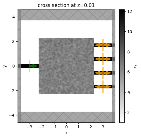
Let’s test out our function. We’ll make an initially random array of parameters between 0 and 1 and generate the static simulation to plot and inspect.
[12]:
np.random.seed(0)  # fix a random seed for reproducibility
params0 = np.random.random((nx, ny))
sim0 = get_sim(params0, beta=beta0)
[13]:
ax = sim0.plot_eps(z=0.01)
ax.set_aspect("equal")
Defining Objective Function#
With our simulation fully defined as a function of our parameters, we are ready to define our objective function.
In this case, it is quite simple, we simply measure the transmitted power in our n=4 output waveguide modes for each of the n=4 design frequencies.
Our objective when looking at waveguide i will be to maximize power transmission at frequency i. To reduce cross talk between waveguide i and frequency j != i, we will subtract the average of the power transmissions for all of the other ports.
Our overall metric will then be the (smooth) minimum.
[14]:
import xarray as xr


def average_over_channel(spectrum: xr.DataArray, fmin: float, fmax: float) -> xr.DataArray:
    """Get average of the spectrum within the frequency range between fmin and fmax."""
    freqs = spectrum.f
    freqs_in_channel = np.logical_and(freqs >= fmin, freqs <= fmax).values
    num_freqs = np.sum(freqs_in_channel)
    avg_power = spectrum.values @ freqs_in_channel / num_freqs
    return avg_power


def get_power(sim_data: td.SimulationData, mnt_index: int, freq_index: int) -> float:
    """Get the average power at waveguide `mnt_index` and frequency channel `freq_index`."""
    mnt_name = mnts_mode[mnt_index].name
    mnt_data = sim_data[mnt_name]
    fmin_channel, fmax_channel = channel_bounds[freq_index]
    amp = mnt_data.amps.sel(direction="+", mode_index=0)
    power_spectrum = anp.abs(amp) ** 2
    return average_over_channel(power_spectrum, fmin=fmin_channel, fmax=fmax_channel)


def get_metric(sim_data: td.SimulationData, mnt_index: int, leak_weight: float = 1.0) -> float:
    """measure of how well this channel (`mnt_index`) performs. With an adjustable weight to reduce cross talk influence."""

    power_all = [
        get_power(sim_data=sim_data, mnt_index=mnt_index, freq_index=j)
        for j in range(num_freqs_design)
    ]

    power_transmitted = power_all[mnt_index]

    # remove the extra term of power_self in power_all
    power_leaked = sum(power_all) - power_transmitted
    avg_power_leaked = power_leaked / (num_freqs_design - 1)

    return power_transmitted - leak_weight * avg_power_leaked
Next we add a penalty to produce structures that are invariant under erosion and dilation, which is a useful approach to implementing minimum length scale features.
[15]:
from tidy3d.plugins.autograd import make_erosion_dilation_penalty

beta_penalty = 10

penalty = make_erosion_dilation_penalty(radius, dl_design_region, beta=beta_penalty)
Total Objective function#
Then we write an objective function that constructs our simulation, runs it, measures our metric, and subtracts our penalty.
[16]:
from tidy3d.plugins.autograd import smooth_min

# useful for debugging, if you want to turn off the metric or the penalty
use_penalty = True
use_metric = True


def objective(params, beta: float, penalty_weight: float = 1.0, leak_weight: float = 0.0) -> float:
    metric = 0.0
    penalty_value = 0.0

    if use_metric:
        sim = get_sim(params, beta=beta, include_extra_mnts=False)
        sim_data = web.run(sim, task_name="autograd9wdm", verbose=False)

        # Calculate the individual metric for each channel
        all_metrics = []
        for mnt_index in range(num_freqs_design):
            metric_i = get_metric(sim_data=sim_data, mnt_index=mnt_index, leak_weight=leak_weight)
            all_metrics.append(metric_i)

        # The objective is the smooth minimum of all channel metrics
        metric = smooth_min(anp.array(all_metrics))

    if use_penalty:
        penalty_value = penalty(params)

    return metric - penalty_weight * penalty_value
Differentiating the objective#
Finally, we can simply use autograd (ag) to transform this objective function into a function that returns our objective function value and our gradient, which we will feed to the optimizer.th
[17]:
grad_fn = ag.value_and_grad(objective)
Let’s try out our gradient function.
[18]:
J, grad = grad_fn(params0, beta=1)
[19]:
print(J)
print(grad.shape)
print(np.linalg.norm(grad))
-2.3312611978128945
(300, 300)
0.034473321359980824
Run Optimization#
Finally, we are ready to optimize our device. We will use Tidy3D’s built-in Adam optimizer in a simple explicit loop, as we’ve done in the previous inverse design tutorials.
We record a history of objective function values, and parameters, for visualization later.
[20]:
from tidy3d.plugins.autograd import adam, apply_updates

# hyperparameters
num_steps = 50
learning_rate = 0.1
beta_min = 1
beta_max = 50

# initialize adam optimizer with starting parameters
params = 0.5 * np.ones_like(params0)

optimizer = adam(learning_rate=learning_rate)
opt_state = optimizer.init(params)

# store history
Js = []
params_history = [np.array(params)]
data_history = []
beta_history = []

for i in range(num_steps):
    perc_done = i / (num_steps - 1)

    # in case we want to change parameters over the optimization procedure

    one_third = 1.0 / 3.0
    # metric = 0.00

    penalty_weight = 1.0
    leak_weight = 0.0 if perc_done < one_third else 1.0
    beta_i = beta_min * (1 - perc_done) + beta_max * perc_done

    # make a plot of density to check on progress
    density = get_density(params, beta_i)
    plt.subplots(figsize=(2, 2))
    plt.imshow(np.flipud(1 - density.T), cmap="gray", vmin=0, vmax=1)
    plt.axis("off")
    plt.show()

    # compute gradient and current objective function value
    value, gradient = grad_fn(
        params, beta=beta_i, penalty_weight=penalty_weight, leak_weight=leak_weight
    )

    # outputs
    print(f"step = {i + 1}")
    print(f"\tJ = {value:.4e}")
    print(f"\tbeta = {beta_i:.2f}")
    print(f"\tgrad_norm = {np.linalg.norm(gradient):.4e}")

    # compute and apply updates to the optimizer based on gradient (-1 sign to maximize obj_fn)
    updates, opt_state = optimizer.update(-gradient, opt_state, params)
    params[:] = apply_updates(params, updates)

    # keep params between 0 and 1
    np.clip(params, 0.0, 1.0, out=params)

    # save history
    Js.append(value)
    params_history.append(params.copy())
    beta_history.append(beta_i)

step = 1
        J = -2.3286e+00
        beta = 1.00
        grad_norm = 3.3650e-02

step = 2
        J = -2.3281e+00
        beta = 2.00
        grad_norm = 4.0105e-02
step = 3
        J = -2.3276e+00
        beta = 3.00
        grad_norm = 6.0303e-02
step = 4
        J = -2.2520e+00
        beta = 4.00
        grad_norm = 8.8373e-02
step = 5
        J = -2.2028e+00
        beta = 5.00
        grad_norm = 9.9900e-02
step = 6
        J = -2.1551e+00
        beta = 6.00
        grad_norm = 6.5487e-02
step = 7
        J = -2.0837e+00
        beta = 7.00
        grad_norm = 8.6697e-02
step = 8
        J = -1.9858e+00
        beta = 8.00
        grad_norm = 1.6983e-01
step = 9
        J = -1.9865e+00
        beta = 9.00
        grad_norm = 9.4289e-02
step = 10
        J = -1.9091e+00
        beta = 10.00
        grad_norm = 9.4493e-02
step = 11
        J = -1.8067e+00
        beta = 11.00
        grad_norm = 1.1012e-01

step = 12
        J = -1.7523e+00
        beta = 12.00
        grad_norm = 1.0648e-01
step = 13
        J = -1.7420e+00
        beta = 13.00
        grad_norm = 1.5391e-01

step = 14
        J = -1.6389e+00
        beta = 14.00
        grad_norm = 7.9687e-02

step = 15
        J = -1.6051e+00
        beta = 15.00
        grad_norm = 1.4281e-01

step = 16
        J = -1.6062e+00
        beta = 16.00
        grad_norm = 1.6201e-01

step = 17
        J = -1.5072e+00
        beta = 17.00
        grad_norm = 1.2868e-01
step = 18
        J = -1.5450e+00
        beta = 18.00
        grad_norm = 1.5561e-01
step = 19
        J = -1.5035e+00
        beta = 19.00
        grad_norm = 1.7985e-01

step = 20
        J = -1.5066e+00
        beta = 20.00
        grad_norm = 2.1237e-01

step = 21
        J = -1.3801e+00
        beta = 21.00
        grad_norm = 1.2513e-01

step = 22
        J = -1.3960e+00
        beta = 22.00
        grad_norm = 2.4046e-01

step = 23
        J = -1.2968e+00
        beta = 23.00
        grad_norm = 1.5136e-01

step = 24
        J = -1.2803e+00
        beta = 24.00
        grad_norm = 1.5617e-01

step = 25
        J = -1.2107e+00
        beta = 25.00
        grad_norm = 1.2141e-01

step = 26
        J = -1.2115e+00
        beta = 26.00
        grad_norm = 1.3964e-01

step = 27
        J = -1.1579e+00
        beta = 27.00
        grad_norm = 1.1888e-01

step = 28
        J = -1.1091e+00
        beta = 28.00
        grad_norm = 8.1777e-02

step = 29
        J = -1.1002e+00
        beta = 29.00
        grad_norm = 1.3578e-01

step = 30
        J = -1.0889e+00
        beta = 30.00
        grad_norm = 1.3518e-01

step = 31
        J = -1.0273e+00
        beta = 31.00
        grad_norm = 1.4102e-01

step = 32
        J = -9.8077e-01
        beta = 32.00
        grad_norm = 1.5798e-01

step = 33
        J = -9.9219e-01
        beta = 33.00
        grad_norm = 1.7487e-01

step = 34
        J = -9.2032e-01
        beta = 34.00
        grad_norm = 1.3297e-01

step = 35
        J = -9.8357e-01
        beta = 35.00
        grad_norm = 2.4761e-01

step = 36
        J = -8.8175e-01
        beta = 36.00
        grad_norm = 1.4976e-01

step = 37
        J = -9.1635e-01
        beta = 37.00
        grad_norm = 1.9233e-01

step = 38
        J = -9.0993e-01
        beta = 38.00
        grad_norm = 2.3617e-01

step = 39
        J = -8.7915e-01
        beta = 39.00
        grad_norm = 2.4549e-01

step = 40
        J = -9.0356e-01
        beta = 40.00
        grad_norm = 3.5707e-01

step = 41
        J = -8.0682e-01
        beta = 41.00
        grad_norm = 1.5621e-01

step = 42
        J = -8.0862e-01
        beta = 42.00
        grad_norm = 1.8145e-01

step = 43
        J = -7.8076e-01
        beta = 43.00
        grad_norm = 1.2660e-01

step = 44
        J = -7.7434e-01
        beta = 44.00
        grad_norm = 1.6875e-01

step = 45
        J = -7.6127e-01
        beta = 45.00
        grad_norm = 1.2395e-01

step = 46
        J = -7.4360e-01
        beta = 46.00
        grad_norm = 7.3564e-02

step = 47
        J = -7.3793e-01
        beta = 47.00
        grad_norm = 9.6975e-02

step = 48
        J = -7.2716e-01
        beta = 48.00
        grad_norm = 8.4624e-02

step = 49
        J = -7.1753e-01
        beta = 49.00
        grad_norm = 5.8642e-02

step = 50
        J = -7.1261e-01
        beta = 50.00
        grad_norm = 7.0499e-02
Visualize Results#
Let’s visualize the results of our optimization.
Objective function vs Iteration#
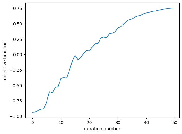
First we inspect the objective function value as a function of optimization iteration number. We see that it steadily increases as expected.
[21]:
plt.plot(Js)
plt.xlabel("iteration number")
plt.ylabel("objective function")
plt.show()
Final Simulation#
Let’s take a look at the final simulation, which we grab from our history.
[22]:
# we'll sample the modes at a finer frequency resolution for this final evaluation, for smoother plots

num_freqs_measure = 151
freqs_measure = np.linspace(freq_min - df_design, freq_max + df_design, num_freqs_measure)

sim_final = get_sim(params_history[-1], beta=beta_history[-1])

for i in range(num_freqs_design):
    sim_final = sim_final.updated_copy(freqs=freqs_measure, path=f"monitors/{i}")
    sim_final = sim_final.updated_copy(freqs=freqs_measure, path=f"monitors/{i + num_freqs_design}")
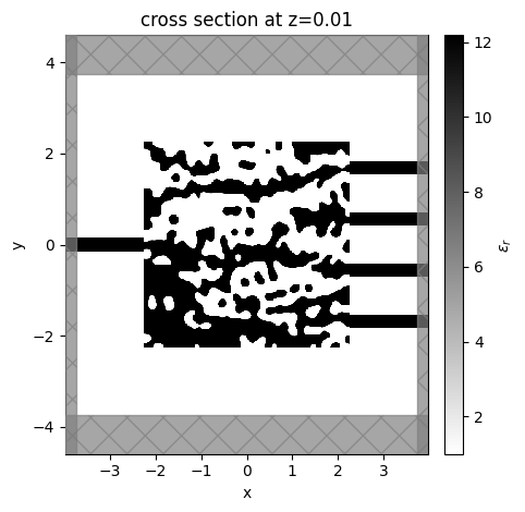
[23]:
ax = sim_final.plot_eps(z=0.01, monitor_alpha=0, source_alpha=0)
[24]:
penalty_value_final = penalty(params_history[-1])
print(penalty_value_final)
0.15197641811046067
[25]:
sim_data_final = web.run(sim_final, task_name="wdm_final")
16:36:49 CET Created task 'wdm_final' with resource_id
             'fdve-b9d8af00-9c5b-49c9-82fd-1727fc95a64b' and task_type 'FDTD'.
             View task using web UI at
             'https://tidy3d.simulation.cloud/workbench?taskId=fdve-b9d8af00-9c5
             b-49c9-82fd-1727fc95a64b'.
Task folder: 'default'.
16:36:59 CET Estimated FlexCredit cost: 0.100. Minimum cost depends on task
             execution details. Use 'web.real_cost(task_id)' to get the billed
             FlexCredit cost after a simulation run.
16:37:01 CET status = queued
             To cancel the simulation, use 'web.abort(task_id)' or
             'web.delete(task_id)' or abort/delete the task in the web UI.
             Terminating the Python script will not stop the job running on the
             cloud.
16:37:08 CET status = preprocess
16:37:13 CET starting up solver
running solver
16:37:28 CET early shutoff detected at 14%, exiting.
status = postprocess
16:37:34 CET status = success
16:37:36 CET View simulation result at
             'https://tidy3d.simulation.cloud/workbench?taskId=fdve-b9d8af00-9c5
             b-49c9-82fd-1727fc95a64b'.
16:37:55 CET Loading results from simulation_data.hdf5
Flux#
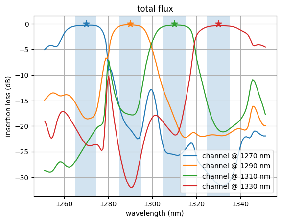
Let’s inspect the flux over each of the output ports as a function of wavelength.
We notice that the ports have peaks in transmission at their corresponding design wavelengths, and are suppressed at the other wavelengths, as expected!
[26]:
for i in range(num_freqs_design):
    freq = freqs_design[i]
    flux_data = sim_data_final[mnts_flux[i].name]
    wvl_nm = 1000 * td.C_0 / freq
    wavelengths_nm = 1000 * td.C_0 / np.array(flux_data.flux.f)
    flux = np.array(flux_data.flux.values)
    loss_db = 10 * np.log10(flux)
    label = f"channel @ {int(wvl_nm)} nm"
    fmin, fmax = channel_bounds[i]
    plt.gca().axvspan(1000 * td.C_0 / fmin, 1000 * td.C_0 / fmax, alpha=0.2)
    plt.plot(wavelengths_nm, loss_db, label=label)
    plt.scatter([wvl_nm], [0], 100, marker="*")
    plt.xlabel("wavelength (nm)")
    plt.ylabel("insertion loss (dB)")
    plt.legend()
    plt.grid("on")
plt.title("total flux")
plt.show()
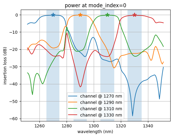
[27]:
for i in range(num_freqs_design):
    freq = freqs_design[i]
    amps = sim_data_final[mnts_mode[i].name].amps
    powers = np.abs(amps.sel(direction="+", mode_index=0)) ** 2
    wvl_nm = 1000 * td.C_0 / freq
    wavelengths_nm = 1000 * td.C_0 / np.array(flux_data.flux.f)
    flux = np.array(powers.values)
    loss_db = 10 * np.log10(flux)
    label = f"channel @ {int(wvl_nm)} nm"
    fmin, fmax = channel_bounds[i]
    plt.gca().axvspan(1000 * td.C_0 / fmin, 1000 * td.C_0 / fmax, alpha=0.2)
    plt.plot(wavelengths_nm, loss_db, label=label)
    plt.scatter([wvl_nm], [0], 100, marker="*")
    plt.xlabel("wavelength (nm)")
    plt.ylabel("insertion loss (dB)")
    plt.legend()
    plt.grid("on")
plt.title("power at mode_index=0")
plt.show()
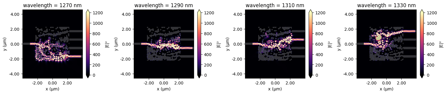
Fields#
Let’s also plot the field intensity patterns at each of the design wavelengths.
We see from this plot the expected result that the power is directed to the design port at each frequency.
[28]:
# plot fields at the two design wavelengths

fig, axes = plt.subplots(
    1, num_freqs_design, tight_layout=True, figsize=(15, 0.8 * num_freqs_design)
)

for freq, ax in zip(freqs_design, axes):
    sim_data_final.plot_field("field", "E", "abs^2", f=freq, ax=ax, vmax=1200)
    wvl = 1000 * td.C_0 / freq
    ax.set_title(f"wavelength = {int(wvl)} nm")
Animation#
Finally, we animate this plot as a function of iteration number. The animation shows the device quickly accomplishing our design objective.
Note: can take a few minutes to complete
[29]:
import matplotlib.animation as animation
from IPython.display import HTML

fig, ax1 = fig, axes = plt.subplots(1, 1, tight_layout=False, figsize=(9, 4))


def animate(i):
    sim_i = get_sim(params_history[i], beta_history[i])
    sim_i.plot_eps(z=0.01, monitor_alpha=0, source_alpha=0, ax=ax1)
    ax1.set_aspect("equal")


# create animation
ani = animation.FuncAnimation(fig, animate, frames=len(beta_history))
plt.close()
[30]:
# display the animation (press "play" to start)
HTML(ani.to_jshtml())
[30]:
<Figure size 640x480 with 0 Axes>
To save the animation as a file, uncomment the line below
Note: can take several more minutes to complete
[31]:
ani.save("img/animation_wdm_autograd.gif", fps=30)
<Figure size 640x480 with 0 Axes>
Export to GDS#
The Simulation object has the .to_gds_file convenience function to export the final design to a GDS file. In addition to a file name, it is necessary to set a cross-sectional plane (z = 0 in this case) on which to evaluate the geometry, a frequency to evaluate the permittivity, and a permittivity_threshold to define the shape boundaries in custom
mediums. See the GDS export notebook for a detailed example on using .to_gds_file and other GDS related functions.
[32]:
sim_final.to_gds_file(
    fname="./misc/inv_des_wdm_ag.gds",
    z=0,
    permittivity_threshold=(n_si**2 + 1) / 2,
    frequency=freq0,
)