Cavity quality factor, effective mode volume, and Purcell factor#
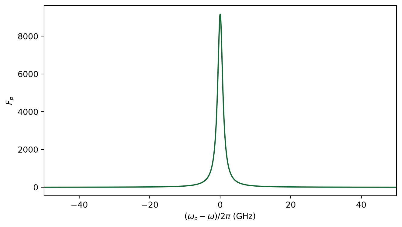
In this notebook, we will walk through the process of calculating the quality factor (\(Q\)), the effective mode volume (\(V_{eff}\)), and the Purcell factor (\(F_{p}\)) of a L3 photonic crystal (PhC) nanocavity. We start by using the Resonance Finder plugin to find the L3 PhC cavity fundamental resonance and extract its
information. For those not familiar with the Resonance Finder, detailed information is available in Extracting resonance information using Resonance Finder, Optimized photonic crystal L3 cavity, or Band structure calculation of a photonic crystal slab notebooks. Then, we
show how to estimate the cavity effective mode volume from the frequency-domain fields. Lastly, the Purcell factor is calculated from the quality factor and the mode effective volume.
If you are new to the finite-difference time-domain (FDTD) method, we highly recommend going through our FDTD101 tutorials.
References#
[1] Peter Lodahl, Sahand Mahmoodian, and Søren Stobbe, "Interfacing single photons and single quantum dots with photonic nanostructures," Rev. Mod. Phys. 87, 347 (2015) DOI: 10.1103/RevModPhys.87.347
[2] R. Coccioli, M. Boroditsky, K.W. Kim, Y. Rahmat-Samii, and E. Yablonovitch, "Smallest possible electromagnetic mode volume in a dielectric cavity," IEE Proceedings - Optoelectronics 145(6), 391 – 397 (1998) DOI: 10.1049/ip-opt:19982468
[3] P. T. Kristensen, C. Van Vlack, and S. Hughes, "Generalized effective mode volume for leaky optical cavities," Opt. Lett. 37, 1649-1651 (2012) DOI: 10.1364/OL.37.001649
[4] Y. Xu, J. S. Vučković, R. K. Lee, O. J. Painter, A. Scherer, and A. Yariv, "Finite-difference time-domain calculation of spontaneous emission lifetime in a microcavity," J. Opt. Soc. Am. B 16, 465-474 (1999) DOI: 10.1364/JOSAB.16.000465
[1]:
# Standard python imports.
import matplotlib.pyplot as plt
import numpy as np

# Tidy3D imports.
import tidy3d as td
import tidy3d.web as web
from tidy3d.plugins.resonance import ResonanceFinder
PhC L3 Cavity Set Up#
To illustrate the calculation of cavity quality factor, effective mode volume, and Purcell factor, we will build an L3 PhC nanocavity. The cavity parameters were obtained from Fig. 23 of [1].
[2]:
# PhC nanocavity geometry.
a = 0.240
r = 0.3 * a
t = 0.6 * a
r_1 = 0.24 * a
d_1 = 0.16 * a
n_x = 21
n_y = 17

# PhC nanocavity material.
n = 3.46
mat_slab = td.Medium(permittivity=n**2)
mat_hole = td.Medium(permittivity=1)

# Simulation wavelength.
wl_min = 0.90
wl_max = 0.92
n_wl = 21
wl_c = (wl_min + wl_max) / 2
wl_range = np.linspace(wl_min, wl_max, n_wl)
freq_c = td.C_0 / wl_c
freq_range = td.C_0 / wl_range
freq_bw = 0.5 * (freq_range[0] - freq_range[-1])

# Simulation runtime.
runtime_fwidth = 20.0  # In units of 1/frequency bandwidth of the source.
t_start_fwidth = (
    2.0  # Time to start monitoring after source has decayed, units of 1/frequency bandwidth.
)
run_time = runtime_fwidth / freq_bw
t_start = t_start_fwidth / freq_bw
print(f"Total runtime = {(run_time * 1e12):.2f} ps")
print(f"Start monitoring fields after {(t_start * 1e12):.2f} ps")
Total runtime = 5.52 ps
Start monitoring fields after 0.55 ps
The following function was adapted from the notebook Defining common photonic crystal structures and is employed to create the L3 PhC nanocavity holes.
[3]:
def hex_l_cavity(
    R: float = 0.26,
    side_R: float = 0.1,
    del_R: float = 0.0,
    spacing_x: float = 0,
    spacing_y: float = 0,
    n_x: int = 34,
    n_y: int = 17,
    height: float = 0.22,
    mat_hole: td.Medium = td.Medium(permittivity=1),
) -> td.Structure:
    # parameters
    # ------------------------------------------------------------
    # R: radius of the cylinders (um)
    # side_R: radii of the two ends of the L-cavity (um)
    # del_R: shift of the two ends of the L-cavity (um)
    # spacing_x: distance between centers of cylinders in x direction (um)
    # spacing_y: distance between centers of cylinders in y direction (um)
    # n_x: number of cylinders in x direction
    # n_y: number of cylinders in y direction
    # height: height of cylinders
    # mat_hole: medium of the PhC cylinders

    x0 = 0  # x coordinate of center of the array (um).
    y0 = 0  # y coordinate of center of the array (um).
    z0 = 0  # z coordinate of center of the array (um).
    l_number = 3  # Number of cylinders removed from center (along x direction).
    reference_plane = "bottom"  # Reference plane.
    sidewall_angle = 0  # Angle slant of cylinders.
    axis = 2  # Cylinders axis.

    cylinders = []
    if n_y % 2 == 0:
        n_y -= 1  # only odd numbers for n_y work for symmetry

    n_middle = n_x - n_x % 2 + l_number % 2

    for i in range(-(n_y // 2), n_y // 2 + 1):  # go up columns
        n_row = (
            n_middle + (i % 2) * (-1) ** l_number
        )  # calculates number of cylinders in current row
        for j in range(-n_row + 1, n_row + 1, 2):  # go along rows
            if i != 0 or abs(j) > l_number:  # don't populate cavity with cylinders
                var_radius = R
                shift_x = 0
                if i == 0 and (abs(j) == l_number + 1):  # checks if cylinder is on side of cavity
                    var_radius = side_R
                    shift_x = del_R * np.sign(j)
                c = td.Cylinder(
                    axis=axis,
                    sidewall_angle=sidewall_angle,
                    reference_plane=reference_plane,
                    radius=var_radius,
                    center=(x0 + j * spacing_x + shift_x, y0 + i * spacing_y, z0),
                    length=height,
                )
                cylinders.append(c)
    structure = td.Structure(geometry=td.GeometryGroup(geometries=cylinders), medium=mat_hole)
    return structure
Next, we will define the PhC structure. We consider a hexagonal lattice to calculate the periodicity in x- and y-directions.
[4]:
# PhC periodicity
p_x = a * np.cos(60 * np.pi / 180)
p_y = a * np.sin(60 * np.pi / 180)

# Simulation size.
pml_gap = 0.6 * wl_max
size_x = 2 * n_x * p_x
size_y = n_y * p_y
size_z = t + 2 * pml_gap
_inf = 10

# PhC slab.
phc_slab = td.Structure(
    geometry=td.Box.from_bounds(
        rmin=(-_inf - size_x / 2, -_inf - size_y / 2, -t / 2),
        rmax=(+_inf + size_x / 2, +_inf + size_y / 2, +t / 2),
    ),
    medium=mat_slab,
)

# PhC holes.
phc_holes = hex_l_cavity(
    R=r,
    side_R=r_1,
    del_R=d_1,
    spacing_x=p_x,
    spacing_y=p_y,
    n_x=n_x,
    n_y=n_y,
    height=t,
    mat_hole=mat_hole,
)
We will include a point dipole at the center of the simulation domain to excite only the fundamental L3 PhC nanocavity mode. The Resonance Finder plugin needs at least one FieldTimeMonitor to record the field as a function of time. Importantly, we start the monitors after the source pulse has decayed.
[5]:
# Point dipole source.
pulse = td.GaussianPulse(freq0=freq_c, fwidth=freq_bw)
dip_source = td.PointDipole(
    source_time=pulse,
    center=(0, 0, 0),
    polarization="Ey",
    name="dip_source",
)

# Field time monitor.
mon_fieldtime = td.FieldTimeMonitor(
    fields=["Ey"],
    center=(0, 0, 0),
    size=(0, 0, 0),
    start=t_start,
    name="monitor_time",
)
In the simulation, we will include a 3D FieldMonitor to calculate the cavity effective mode volume. We have obtained the resonance frequency from a previous simulation.
[6]:
# Mode resonance frequency.
mode_freq = freq_c

# Apodization to exclude the source pulse from the frequency-domain monitors.
apod = td.ApodizationSpec(start=t_start, width=t_start / 10)

# Field monitor.
mon_box = td.Box(center=(0, 0, 0), size=(size_x / 2, size_y / 2, 4 * t))
mon_field = td.FieldMonitor(
    center=mon_box.center,
    size=mon_box.size,
    freqs=mode_freq,
    name="field_vol",
    colocate=False,
    apodization=apod,
)

eps_mon = td.PermittivityMonitor(
    center=mon_box.center, size=mon_box.size, freqs=mode_freq, name="eps_mon", colocate=False
)
Now, we can build and run the simulation. It is worth mentioning that we set shutoff=0 to run the simulation only for the run_time period. Otherwise, the simulation can take a very long time for the fields to decay fully.
[7]:
sim = td.Simulation(
    center=(0, 0, 0),
    size=(size_x, size_y, size_z),
    grid_spec=td.GridSpec.auto(wavelength=wl_c, min_steps_per_wvl=20),
    structures=[phc_slab, phc_holes],
    sources=[dip_source],
    monitors=[mon_fieldtime, mon_field, eps_mon],
    run_time=run_time,
    shutoff=0,
    boundary_spec=td.BoundarySpec.all_sides(boundary=td.PML()),
    normalize_index=None,
    symmetry=(1, -1, 1),
)

sim.plot_3d(width=400, height=400)
07:51:33 UTC WARNING: Structure: simulation.structures[1] (no `name` was
             specified) was detected as being less than half of a central
             wavelength from a PML on side x-min. To avoid inaccurate results or
             divergence, please increase gap between any structures and PML or
             fully extend structure through the pml.
WARNING: Suppressed 3 WARNING messages.
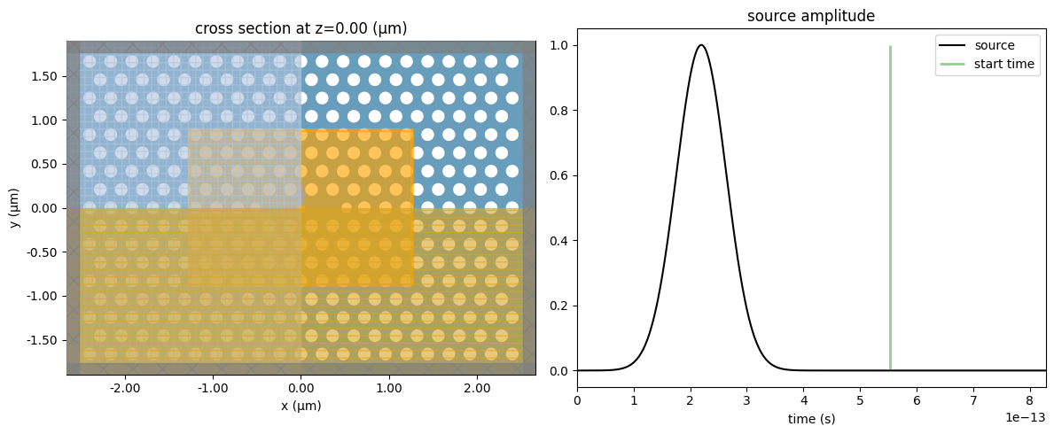
Before running the simulation, let’s look at the source and monitor positions to certify we are measuring the fields after the sources have fully decayed.
[8]:
fig, (ax1, ax2) = plt.subplots(1, 2, tight_layout=True, figsize=(12, 5))
sim.plot(z=0.0, ax=ax1)

plot_time = 3 / freq_bw
sim.sources[0].source_time.plot(times=np.linspace(0, plot_time, 1001), val="abs", ax=ax2)
ax2.set_xlim(0, plot_time)
ax2.vlines(t_start, 0, 1, linewidth=2, color="g", alpha=0.4)
ax2.legend(["source", "start time"])
plt.show()
Now, let’s run the simulation!
[9]:
job = web.Job(simulation=sim, task_name="l3_nanocavity", verbose=True)
sim_data = job.run(path="data/simulation_data.hdf5")
07:51:34 UTC WARNING: Structure: simulation.structures[1] (no `name` was
             specified) was detected as being less than half of a central
             wavelength from a PML on side x-min. To avoid inaccurate results or
             divergence, please increase gap between any structures and PML or
             fully extend structure through the pml.
WARNING: Suppressed 3 WARNING messages.
             WARNING: Structure: simulation.structures[1] (no `name` was
             specified) was detected as being less than half of a central
             wavelength from a PML on side x-min. To avoid inaccurate results or
             divergence, please increase gap between any structures and PML or
             fully extend structure through the pml.
WARNING: Suppressed 3 WARNING messages.
07:51:35 UTC WARNING: Structure: simulation.structures[1] (no `name` was
             specified) was detected as being less than half of a central
             wavelength from a PML on side x-min. To avoid inaccurate results or
             divergence, please increase gap between any structures and PML or
             fully extend structure through the pml.
WARNING: Suppressed 3 WARNING messages.
             Created task 'l3_nanocavity' with resource_id
             'fdve-1589606d-0e28-41ca-8b3f-296e21f2ebcc' and task_type 'FDTD'.
             View task using web UI at
             'https://tidy3d.simulation.cloud/workbench?taskId=fdve-1589606d-0e2
             8-41ca-8b3f-296e21f2ebcc'.
Task folder: 'default'.
07:52:07 UTC Estimated FlexCredit cost: 0.086. This assumes the FDTD solver runs
             for the full simulation time; if early shutoff is reached, the
             billed cost can be lower. Use 'web.real_cost(task_id)' to get the
             billed FlexCredit cost after a simulation run.
07:52:09 UTC status = queued
             To cancel the simulation, use 'web.abort(task_id)' or
             'web.delete(task_id)' or abort/delete the task in the web UI.
             Terminating the Python script will not stop the job running on the
             cloud.
07:52:25 UTC starting up solver
running solver
07:53:39 UTC status = postprocess
07:53:42 UTC status = success
07:53:44 UTC View simulation result at
             'https://tidy3d.simulation.cloud/workbench?taskId=fdve-1589606d-0e2
             8-41ca-8b3f-296e21f2ebcc'.
07:53:45 UTC Loading results from data/simulation_data.hdf5
07:53:46 UTC WARNING: Structure: simulation.structures[1] (no `name` was
             specified) was detected as being less than half of a central
             wavelength from a PML on side x-min. To avoid inaccurate results or
             divergence, please increase gap between any structures and PML or
             fully extend structure through the pml.
WARNING: Suppressed 3 WARNING messages.
             WARNING: Warning messages were found in the solver log. For more
             information, check 'SimulationData.log' or use
             'web.download_log(task_id)'.
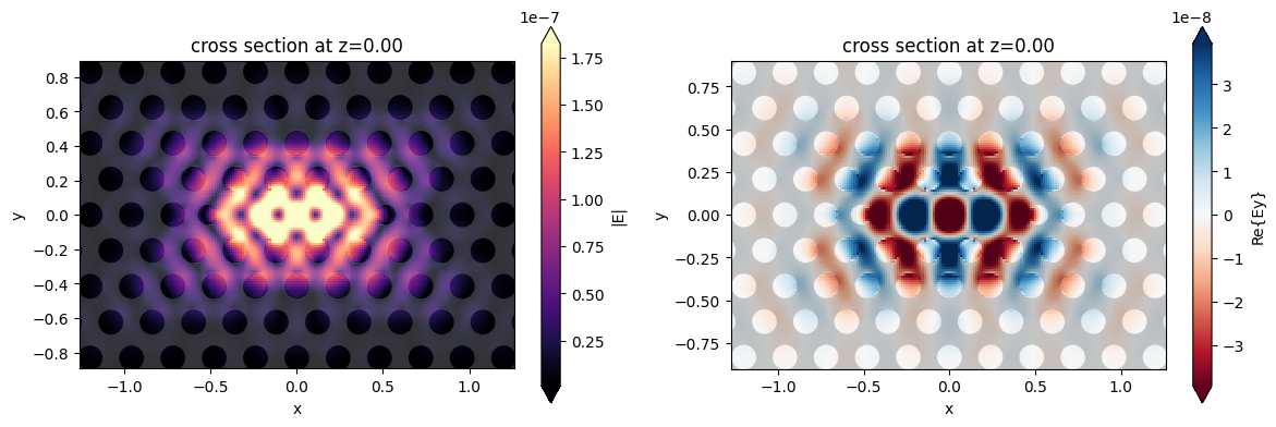
Cavity Field Distribution#
After running the simulation, we can obtain the frequency-domain fields to see what the cavity mode looks like. It is worth mentioning that frequency-domain results are considered accurate only if we run the simulation until the time-domain fields completely decays within the monitor region.
[10]:
fig, (ax1, ax2) = plt.subplots(1, 2, tight_layout=True, figsize=(12, 4))

sim_data.plot_field("field_vol", "E", "abs", z=0, ax=ax1)
sim_data.plot_field("field_vol", "Ey", "real", z=0, ax=ax2)
plt.show()
Quality Factor#
Now, we can analyze the simulation data and calculate the resonance information from the time domain fields. The run() method returns an xr.Dataset containing the decay rate, Q-factor, amplitude, phase, and estimation error.
[11]:
resonance_finder = ResonanceFinder(freq_window=(freq_range[-1], freq_range[0]))
resonance_data = resonance_finder.run(signals=sim_data["monitor_time"])
resonance_data.to_dataframe()