Dielectric metasurface absorber#
Metamaterials and metasurfaces can achieve functionalities that are not available to naturally occurring materials such as negative refractive index. Originally, metamaterials often utilize metallic structures. These metallic structures, such as split ring resonators, exhibit strong resonances at specific frequencies, which can be effectively tuned by adjusting the geometric parameters. However, metals exhibit large loss at optical frequencies. This can greatly impair the performance of the metamaterials. As a consequence, metamaterials fully based on dielectric materials have attracted a lot of interest recently.
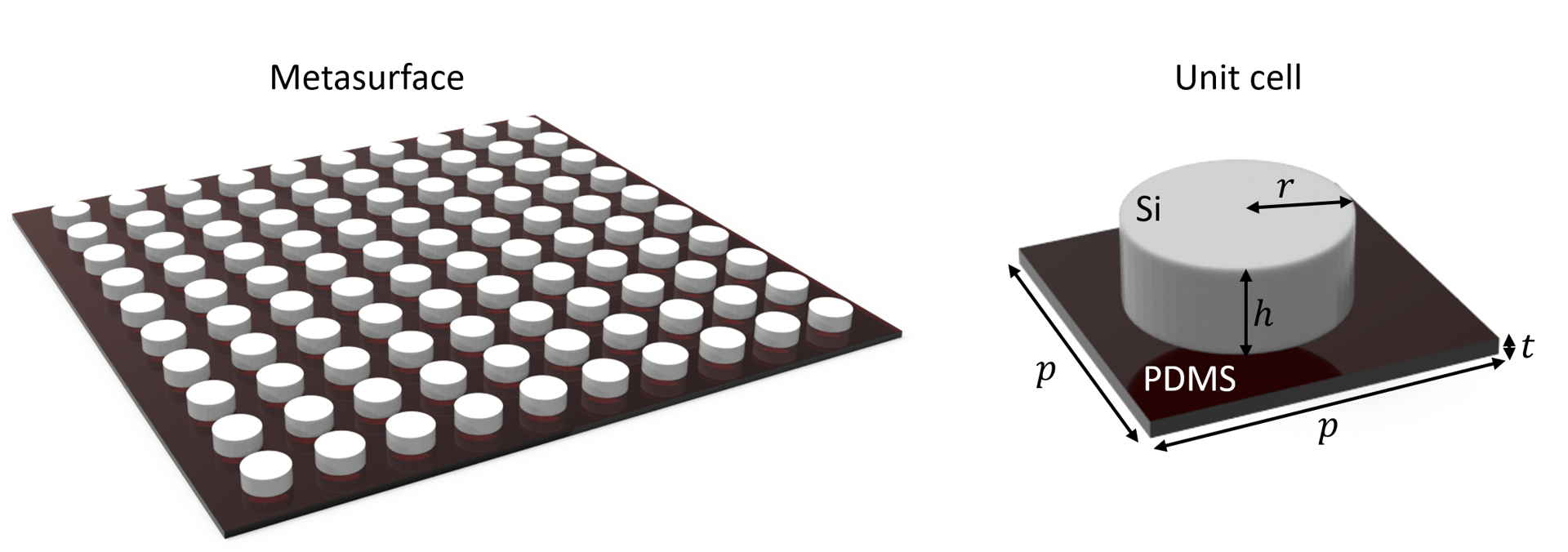
Electromagnetic absorber is one of the most popular categories of metasurfaces. Metasurfaces with high absorption can be used as radiation power detectors since they convert electromagnetic radiation into thermal energy at high efficiency. This model demonstrates how to simulate an all-dielectric metasurface absorber at the THz regime. The design consists of a cylindrical silicon resonator on a thin PDMS substrate. The design parameters are adapted from Kebin Fan, Jonathan Y. Suen, Xinyu Liu, and Willie J. Padilla, “All-dielectric metasurface absorbers for uncooled terahertz imaging,” Optica 4, 601-604 (2017).
In Tidy3D’s example library, we have demonstrated a gradient metasurface reflector, a metalens at the visible frequency, and a graphene metamaterial absorber. In addition, we also investigated a frequency selected surface for the microwave frequency range.
If you are new to the finite-difference time-domain (FDTD) method, we highly recommend going through our FDTD101 tutorials. FDTD simulations can diverge due to various reasons. If you run into any simulation divergence issues, please follow the steps outlined in our troubleshooting guide to resolve it.
[1]:
import matplotlib.pyplot as plt
import numpy as np
import tidy3d as td
import tidy3d.web as web
Simulation Setup#
The absorption peak of the metasurface is designed to be around 0.6 THz. Therefore, we aim to simulate a frequency range from 0.4 THz to 0.8 THz.
[2]:
THz = 1e12  # conversion factor from Hz to THz
freqs = np.linspace(0.4 * THz, 0.8 * THz, 100)  # frequency range of the simulation
freq0 = 0.6 * THz  # central frequency
freqw = 0.4 * THz  # width of the frequency range
lda0 = td.C_0 / freq0  # central wavelength
Two materials are involved in this model. The dielectric cylinder is made of silicon, which is described by a Drude model with \(\varepsilon_{\inf}\)=11.7 and plasma frequency \(\omega_P\)=0.69 THz and damping rate \(\gamma\)=0.83 THz. We can use the built-in Drude feature to describe the response of silicon. The thin substrate is made of PDMS, which has a relative
permittivity of 1.72 and a loss tangent of 0.15 at the relevant frequency range. The relative permittivity and loss tangent will be converted to the complex refractive index then PDMS can be described by using the from_nk method of Medium. Note that this is only strictly accurate at the specified frequency. To ensure it’s accurate at all frequencies, one needs to perform a dispersive material
fitting procedure.
[3]:
w_p = 0.69 * THz  # plasma frequency of Si
gamma = 0.83 * THz  # damping rate of Si
Si = td.Drude(
    eps_inf=11.7, coeffs=[(w_p, gamma)]
)  # using drude model to describe the response of silicon

loss_tan = 0.15  # loss tangent of PDMS
eps_pdms = 1.72 + 1j * 1.72 * loss_tan  # complex permittivity of PDMS
n_pdms = np.sqrt(eps_pdms)  # refractive index of PDMS
PDMS = td.Medium.from_nk(
    n=np.real(n_pdms), k=np.imag(n_pdms), freq=freq0
)  # define PDMS with the complex refractive index
The unit cell of the metasurface consists of a cylindrical silicon resonator on a thin PDMS substrate. The periodicity is 330 \(\mu m\). The cylinder radius and height are 106 \(\mu m\) and 85 \(\mu m\), respectively. The substrate is only 8 \(\mu m\) thick.
[4]:
p = 330  # unit cell size
h = 85  # height of the cylinder
r = 106  # radius of the cylinder
t = 8  # thickness of the substrate
Define the simulation domain and the unit cell structure.
[5]:
# simulation domain size
# simulation size is the periodicity of the unit cell in x and y directions
# in z direction, the size is set to 2 central wavelength
Lx, Ly, Lz = p, p, 2 * lda0
sim_size = [Lx, Ly, Lz]

# construct the pdms substrate
substrate = td.Structure(
    geometry=td.Box(center=[0, 0, -t / 2], size=[td.inf, td.inf, t]), medium=PDMS
)

# construct the silicon resonator
cylinder = td.Structure(
    geometry=td.Cylinder(center=[0, 0, h / 2], radius=r, length=h, axis=2), medium=Si
)
The metasurface is excited by a plane wave at normal incidence. To measure the transmission, reflection, and absorption, we set up two flux monitors, one on the incident side and one on the transmission side. An additional field monitor is added so that we can visualize the resonance mode profile at the absorption peak.
[6]:
# add a plane wave source
plane_wave = td.PlaneWave(
    source_time=td.GaussianPulse(freq0=freq0, fwidth=0.5 * freqw),
    size=(td.inf, td.inf, 0),
    center=(0, 0, 0.3 * lda0),
    direction="-",
    pol_angle=0,
)

# add a flux monitor to detect transmission
monitor_t = td.FluxMonitor(
    center=[0, 0, -0.4 * Lz], size=[td.inf, td.inf, 0], freqs=freqs, name="T"
)

# add a flux monitor to detect reflection
monitor_r = td.FluxMonitor(center=[0, 0, 0.4 * Lz], size=[td.inf, td.inf, 0], freqs=freqs, name="R")

# add a field monitor to see the field profile at the absorption peak frequency
monitor_field = td.FieldMonitor(
    center=[0, 0, 0], size=[td.inf, 0, lda0], freqs=[freq0], name="field"
)
Set up the Simulation object. Using an automatic nonuniform grid is the most efficient and convenient. We set min_steps_per_wvl=40 to ensure it resolves the structure well.
[7]:
run_time = 3e-10  # simulation run time

# set up simulation
sim = td.Simulation(
    size=sim_size,
    grid_spec=td.GridSpec.auto(min_steps_per_wvl=40, wavelength=lda0),
    structures=[substrate, cylinder],
    sources=[plane_wave],
    monitors=[monitor_t, monitor_r, monitor_field],
    run_time=run_time,
    boundary_spec=td.BoundarySpec(
        x=td.Boundary.periodic(), y=td.Boundary.periodic(), z=td.Boundary.pml()
    ),
    symmetry=(-1, 1, 0),
)  # symmetry can be used to greatly reduce the computational cost
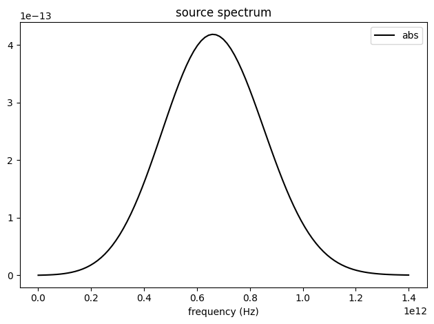
Before submitting the simulation job to the server, it is always a good practice to verify if the settings are correct. For example, we can check if the frequency spectrum of the source covers the frequency range of interest. To do so, we can simply plot it. Here, we need to make sure the time domain sampling is sufficiently fine so we use 2000 points.
[8]:
sim.sources[0].source_time.plot_spectrum(times=np.linspace(0, sim.run_time, 2000), val="abs")
plt.show()
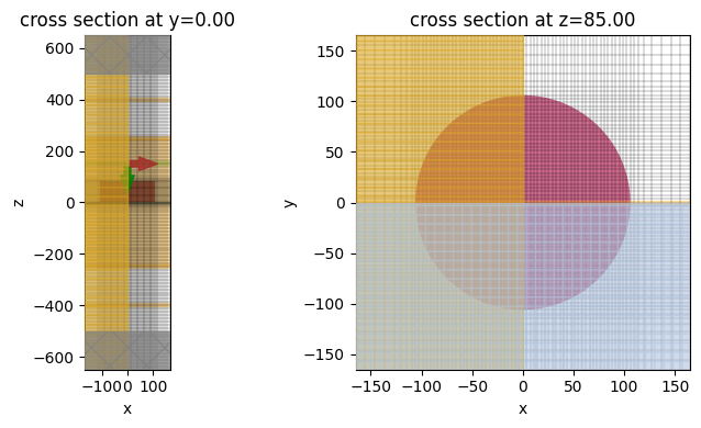
Lastly, to ensure the geometry and mesh are set up appropriately, we visualize them before running the simulation.
[9]:
fig, (ax1, ax2) = plt.subplots(1, 2, tight_layout=True, figsize=(10, 4))
ax1 = sim.plot(y=0, ax=ax1)
ax1 = sim.plot_grid(y=0, ax=ax1)

ax2 = sim.plot(z=h, ax=ax2)
ax2 = sim.plot_grid(z=h, ax=ax2)
To have a better visualization, we can also plot the simulation in 3D.
[10]:
sim.plot_3d()
Running Simulation#
Submit the simulation to the server.
[11]:
sim_data = web.run(
    sim, task_name="all_dielectric_metasurface_absorber", path="data/simulation.hdf5"
)
20:00:13 CEST Created task 'all_dielectric_metasurface_absorber' with task_id
              'fdve-cd88a88e-0bec-43d4-92b2-6ba9ea753157' and task_type 'FDTD'.
              View task using web UI at
              'https://tidy3d.simulation.cloud/workbench?taskId=fdve-cd88a88e-0b
              ec-43d4-92b2-6ba9ea753157'.
Task folder: 'default'.
20:00:15 CEST Maximum FlexCredit cost: 0.025. Minimum cost depends on task
              execution details. Use 'web.real_cost(task_id)' to get the billed
              FlexCredit cost after a simulation run.
20:00:16 CEST status = queued
              To cancel the simulation, use 'web.abort(task_id)' or
              'web.delete(task_id)' or abort/delete the task in the web UI.
              Terminating the Python script will not stop the job running on the
              cloud.
20:01:58 CEST starting up solver
running solver
20:02:02 CEST early shutoff detected at 64%, exiting.
status = postprocess
20:02:04 CEST status = success
20:02:06 CEST View simulation result at
              'https://tidy3d.simulation.cloud/workbench?taskId=fdve-cd88a88e-0b
              ec-43d4-92b2-6ba9ea753157'.
20:02:08 CEST loading simulation from data/simulation.hdf5
Result Visualization#
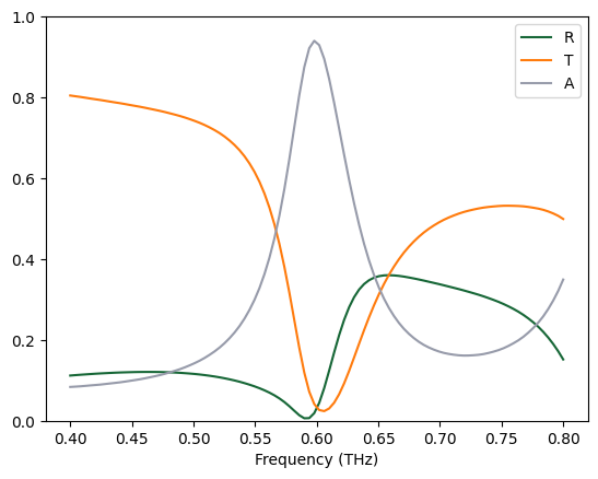
After the simulation is complete, we visualize the reflectance, transmittance, and absorptance spectra. The absorption peak is observed around 0.6 THz as expected. The maximum absorption is around 95%.
[12]:
R = sim_data["R"].flux
T = -sim_data["T"].flux
A = 1 - R - T
freq_thz = np.linspace(0.4, 0.8, 100)
plt.plot(freq_thz, R, freq_thz, T, freq_thz, A)
plt.xlabel("Frequency (THz)")
plt.ylim(0, 1)
plt.legend(("R", "T", "A"))
plt.show()
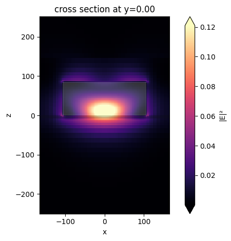
Finally, we visualize the field intensity distribution at the resonance frequency. A strongly localized field within the silicon cylinder is observed, which indicates a high power dissipation due to the resonance mode of the cylinder.
[13]:
sim_data.plot_field(field_monitor_name="field", field_name="E", val="abs^2")
plt.show()
Finite Array of Unit Cells#
The periodic boundary condition indicates that the metasurface is infinitely large in the simulation. In practice, the fabricated metasurface is of course always made of only a finite number of unit cells. In addition, the spot size of the incident light is also finite. Therefore, only a certain number of unit cells are illuminated.
Due to the above mentioned reasons, the transmission, reflection, or absorption spectrum might deviate from the perfectly periodic case. In this section, we model a finite array of unit cells illuminated by a focused Gaussian beam. Thanks to the highly optimized Tidy3D solver, such a large structure can be simulated with ease.
[14]:
Nx = 15 # number of unit cells in the x direction
Ny = 15 # number of unit cells in the y direction
buffer = 0.5 * lda0 # buffer spacing in the x and y directions
# simulation domain size
Lx, Ly, Lz = Nx * p + 2 * buffer, Ny * p + 2 * buffer, 2 * lda0
sim_size = [Lx, Ly, Lz]
# systematically construct the silicon resonators
metasurface = [substrate]
for i in range(Nx):
for j in range(Ny):
cylinder = td.Structure(
geometry=td.Cylinder(center=[i * p, j * p, h / 2], radius=r, length=h, axis=2),
medium=Si,
)
metasurface.append(cylinder)
# define a gaussian beam with a waist radius of 3 wavelengths (focused beam)
gaussian = td.GaussianBeam(
size=(td.inf, td.inf, 0),
source_time=td.GaussianPulse(freq0=freq0, fwidth=0.5 * freqw),
center=(p * (Nx // 2), p * (Ny // 2), 0.3 * lda0),
direction="-",
waist_radius=3 * lda0,
)
# define a field monitor to visualize the field distribution under gaussian beam excitation
monitor_field = td.FieldMonitor(
center=[0, 0, 0], size=[td.inf, td.inf, 0], freqs=[freq0], name="field"
)
sim = td.Simulation(
size=sim_size,
center=(p * (Nx // 2), p * (Ny // 2), 0),
grid_spec=td.GridSpec.auto(min_steps_per_wvl=30, wavelength=lda0),
structures=metasurface,
sources=[gaussian],
monitors=[
monitor_t,
monitor_r,
monitor_field,
], # we will reuse the flux monitors defined earlier
run_time=run_time,
boundary_spec=td.BoundarySpec.all_sides(boundary=td.PML()), # pml is applied in all boundaries
symmetry=(-1, 1, 0),
) # the same symmetry can be used
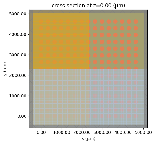
sim.plot(z=0)
plt.show()
[15]:
sim_data = web.run(
    sim,
    task_name="all_dielectric_metasurface_absorber",
    path="data/simulation.hdf5",
    verbose=True,
)
20:02:09 CEST Created task 'all_dielectric_metasurface_absorber' with task_id
              'fdve-5bb6ccf8-c242-4b67-8d06-492efa65f090' and task_type 'FDTD'.
              View task using web UI at
              'https://tidy3d.simulation.cloud/workbench?taskId=fdve-5bb6ccf8-c2
              42-4b67-8d06-492efa65f090'.
Task folder: 'default'.
20:02:11 CEST Maximum FlexCredit cost: 0.324. Minimum cost depends on task
              execution details. Use 'web.real_cost(task_id)' to get the billed
              FlexCredit cost after a simulation run.
20:02:12 CEST status = queued
              To cancel the simulation, use 'web.abort(task_id)' or
              'web.delete(task_id)' or abort/delete the task in the web UI.
              Terminating the Python script will not stop the job running on the
              cloud.
20:11:34 CEST status = preprocess
20:11:39 CEST starting up solver
running solver
20:11:52 CEST early shutoff detected at 20%, exiting.
status = postprocess
20:11:55 CEST status = success
20:11:57 CEST View simulation result at
              'https://tidy3d.simulation.cloud/workbench?taskId=fdve-5bb6ccf8-c2
              42-4b67-8d06-492efa65f090'.
20:12:00 CEST loading simulation from data/simulation.hdf5
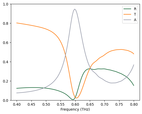
After the simulation is complete, we visualize the reflectance, transmittance, and absorptance spectra in the same way. The spectra are similar to that obtained from the unit cell simulation with only minor differences. This result also verifies the validity of the unit cell simulation with the periodic condition.
[16]:
R = sim_data["R"].flux
T = -sim_data["T"].flux
A = 1 - R - T
freq_thz = np.linspace(0.4, 0.8, 100)
plt.plot(freq_thz, R, freq_thz, T, freq_thz, A)
plt.xlabel("Frequency (THz)")
plt.ylim(0, 1)
plt.legend(("R", "T", "A"))
plt.show()
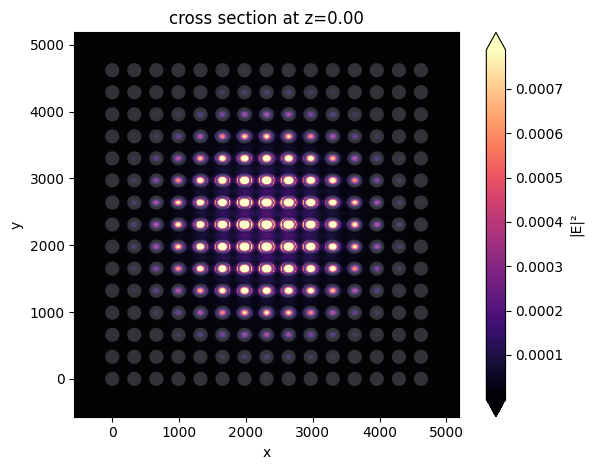
The field intensity distribution reveals that only a small number of unit cells are excited by the gaussian beam.
[17]:
sim_data.plot_field(field_monitor_name="field", field_name="E", val="abs^2")
plt.show()