Performing parallel / batch processing of simulations#
Note: the cost of running the entire notebook is larger than 1 FlexCredit.
In this notebook, we will show an example of using tidy3d to evaluate device performance over a set of many design parameters.
This example will also provide a walkthrough of Tidy3D’s Job and Batch features for managing both individual simulations and sets of simulations.
Note: as of version
2.10, the tidy3d.web.run unifies the submission of a single simulation as well as any nested combination of lists, tuples, and dictionaries of them, handling the same functionality as the batch, with a simpler syntax. As such, it could be a good alternative for parameter scan depending on how your script is set up.
Additionally, we will show how to do this problem using tidy3d.plugins.design, which provides convenience methods for defining and running parameter scans, which has a full tutorial here.
For demonstration, we look at the splitting ratio of a directional coupler as we vary the coupling length between two waveguides. The sidewall of the waveguides is slanted, deviating from the vertical direction by sidewall_angle.
[1]:
# standard python imports
import os

import gdstk
import matplotlib.pyplot as plt
import numpy as np

# tidy3D imports
import tidy3d as td
from tidy3d import web

td.config.logging.level = "ERROR"
Setup#
First we set up some global parameters
[2]:
# wavelength / frequency
lambda0 = 1.550  # all length scales in microns
freq0 = td.constants.C_0 / lambda0
fwidth = freq0 / 10

# Permittivity of waveguide and substrate
wg_n = 3.48
sub_n = 1.45
mat_wg = td.Medium(permittivity=wg_n**2)
mat_sub = td.Medium(permittivity=sub_n**2)

# Waveguide dimensions

# Waveguide height
wg_height = 0.22
# Waveguide width
wg_width = 0.45
# Waveguide separation in the beginning/end
wg_spacing_in = 8
# Reference plane where the cross section of the device is defined
reference_plane = "bottom"
# Angle of the sidewall deviating from the vertical ones, positive values for the base larger than the top
sidewall_angle = np.pi / 6
# Total device length along propagation direction
device_length = 100
# Length of the bend region
bend_length = 16
# space between waveguide and PML
pml_spacing = 1
# resolution control: minimum number of grid cells per wavelength in each material
grid_cells_per_wvl = 16
Define waveguide bends and coupler#
Here is where we define our directional coupler shape programmatically in terms of the geometric parameters
[3]:
def tanh_interp(max_arg):
    """Interpolator for tanh with adjustable extension"""
    scale = 1 / np.tanh(max_arg)
    return lambda u: 0.5 * (1 + scale * np.tanh(max_arg * (u * 2 - 1)))


def make_coupler(
    length,
    wg_spacing_in,
    wg_width,
    wg_spacing_coup,
    coup_length,
    bend_length,
):
    """Make an integrated coupler using the gdstk RobustPath object."""
    # bend interpolator
    interp = tanh_interp(3)
    delta = wg_width + wg_spacing_coup - wg_spacing_in
    offset = lambda u: wg_spacing_in + interp(u) * delta

    coup = gdstk.RobustPath(
        (-0.5 * length, 0),
        (wg_width, wg_width),
        wg_spacing_in,
        simple_path=True,
        layer=1,
        datatype=[0, 1],
    )
    coup.segment((-0.5 * coup_length - bend_length, 0))
    coup.segment(
        (-0.5 * coup_length, 0),
        offset=[lambda u: -0.5 * offset(u), lambda u: 0.5 * offset(u)],
    )
    coup.segment((0.5 * coup_length, 0))
    coup.segment(
        (0.5 * coup_length + bend_length, 0),
        offset=[lambda u: -0.5 * offset(1 - u), lambda u: 0.5 * offset(1 - u)],
    )
    coup.segment((0.5 * length, 0))
    return coup
Create Simulation and Submit Job#
The following function creates a tidy3d simulation object for a set of design parameters.
Note that the simulation has not been run yet, just created.
[4]:
def make_sim(coup_length, wg_spacing_coup, domain_field=False):
    """Make a simulation with a given length of the coupling region and
    distance between the waveguides in that region. If ``domain_field``
    is True, a 2D in-plane field monitor will be added.
    """

    # Geometry must be placed in GDS cells to import into Tidy3D
    coup_cell = gdstk.Cell("Coupler")

    substrate = gdstk.rectangle(
        (-device_length / 2, -wg_spacing_in / 2 - 10),
        (device_length / 2, wg_spacing_in / 2 + 10),
        layer=0,
    )
    coup_cell.add(substrate)

    # Add the coupler to a gdstk cell
    gds_coup = make_coupler(
        device_length,
        wg_spacing_in,
        wg_width,
        wg_spacing_coup,
        coup_length,
        bend_length,
    )
    coup_cell.add(gds_coup)

    # Substrate
    (oxide_geo,) = td.PolySlab.from_gds(
        gds_cell=coup_cell,
        gds_layer=0,
        gds_dtype=0,
        slab_bounds=(-10, 0),
        reference_plane=reference_plane,
        axis=2,
    )

    oxide = td.Structure(geometry=oxide_geo, medium=mat_sub)

    # Waveguides (import all datatypes if gds_dtype not specified)
    coupler1_geo, coupler2_geo = td.PolySlab.from_gds(
        gds_cell=coup_cell,
        gds_layer=1,
        slab_bounds=(0, wg_height),
        sidewall_angle=sidewall_angle,
        reference_plane=reference_plane,
        axis=2,
    )

    coupler1 = td.Structure(geometry=coupler1_geo, medium=mat_wg)

    coupler2 = td.Structure(geometry=coupler2_geo, medium=mat_wg)

    # Simulation size along propagation direction
    sim_length = 2 + 2 * bend_length + coup_length

    # Spacing between waveguides and PML
    sim_size = [
        sim_length,
        wg_spacing_in + wg_width + 2 * pml_spacing,
        wg_height + 2 * pml_spacing,
    ]

    # source
    src_pos = -sim_length / 2 + 0.5
    msource = td.ModeSource(
        center=[src_pos, wg_spacing_in / 2, wg_height / 2],
        size=[0, 3, 2],
        source_time=td.GaussianPulse(freq0=freq0, fwidth=fwidth),
        direction="+",
        mode_spec=td.ModeSpec(),
        mode_index=0,
    )

    mon_in = td.ModeMonitor(
        center=[(src_pos + 0.5), wg_spacing_in / 2, wg_height / 2],
        size=[0, 3, 2],
        freqs=[freq0],
        mode_spec=td.ModeSpec(),
        name="in",
    )
    mon_ref_bot = td.ModeMonitor(
        center=[(src_pos + 0.5), -wg_spacing_in / 2, wg_height / 2],
        size=[0, 3, 2],
        freqs=[freq0],
        mode_spec=td.ModeSpec(),
        name="reflect_bottom",
    )
    mon_top = td.ModeMonitor(
        center=[-(src_pos + 0.5), wg_spacing_in / 2, wg_height / 2],
        size=[0, 3, 2],
        freqs=[freq0],
        mode_spec=td.ModeSpec(),
        name="top",
    )
    mon_bot = td.ModeMonitor(
        center=[-(src_pos + 0.5), -wg_spacing_in / 2, wg_height / 2],
        size=[0, 3, 2],
        freqs=[freq0],
        mode_spec=td.ModeSpec(),
        name="bottom",
    )
    monitors = [mon_in, mon_ref_bot, mon_top, mon_bot]

    if domain_field:
        domain_monitor = td.FieldMonitor(
            center=[0, 0, wg_height / 2],
            size=[td.inf, td.inf, 0],
            freqs=[freq0],
            name="field",
        )
        monitors.append(domain_monitor)

    # initialize the simulation
    sim = td.Simulation(
        size=sim_size,
        grid_spec=td.GridSpec.auto(min_steps_per_wvl=grid_cells_per_wvl),
        structures=[oxide, coupler1, coupler2],
        sources=[msource],
        monitors=monitors,
        run_time=50 / fwidth,
        boundary_spec=td.BoundarySpec.all_sides(boundary=td.PML()),
    )

    return sim
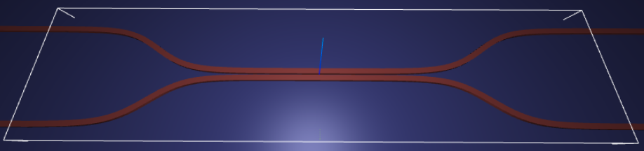
Inspect Simulation#
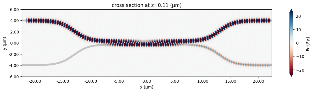
Let’s create and inspect a single simulation to make sure it was defined correctly before doing the full scan. The sidewalls of the waveguides deviate from the vertical direction by 30 degrees. We also add an in-plane field monitor to have a look at the field evolution in this one simulation. We will not use such a monitor in the batch to avoid storing unnecessarily large amounts of data.
[5]:
# Length of the coupling region
coup_length = 10

# Waveguide separation in the coupling region
wg_spacing_coup = 0.10

sim = make_sim(coup_length, wg_spacing_coup, domain_field=True)
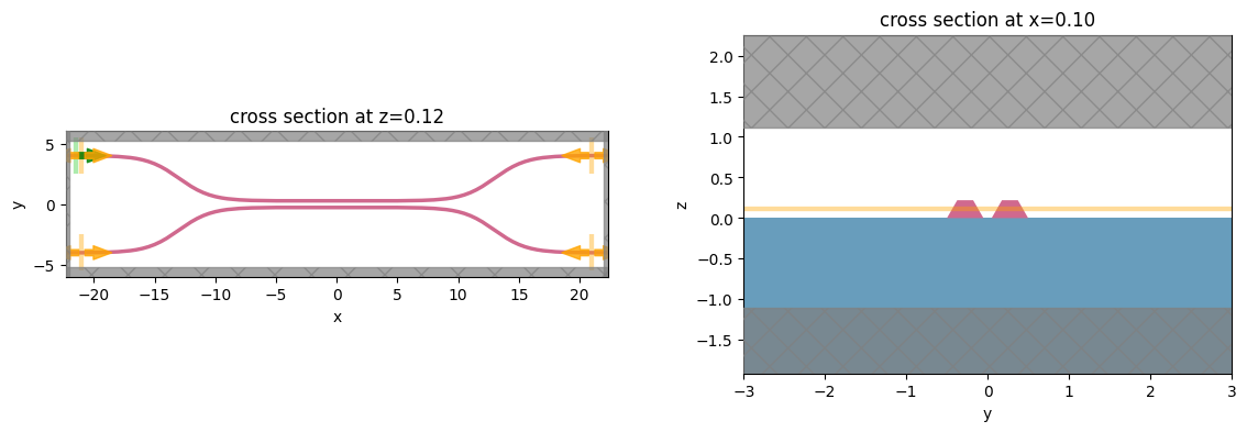
[6]:
# visualize geometry
fig, (ax1, ax2) = plt.subplots(1, 2, figsize=(14, 4))
sim.plot(z=wg_height / 2 + 0.01, ax=ax1)
sim.plot(x=0.1, ax=ax2)
ax2.set_xlim([-3, 3])
plt.show()
Create and Submit Job#
The Job object provides an interface for managing simulations.
job = Job(simulation) will create a job and upload the simulation to our server to run.
Then, one may call various methods of job to monitor progress, download results, and get information.
For more information, refer to the API reference.
[7]:
# create job, upload sim to server to begin running
job = web.Job(simulation=sim, task_name="CouplerVerify", verbose=True)

# download the results and load them into a simulation
sim_data = job.run(path="data/sim_data.hdf5")
07:53:00 UTC Created task 'CouplerVerify' with resource_id
             'fdve-2d7d00e6-22f2-43f9-ac38-24079a0c2531' and task_type 'FDTD'.
             View task using web UI at
             'https://tidy3d.simulation.cloud/workbench?taskId=fdve-2d7d00e6-22f
             2-43f9-ac38-24079a0c2531'.
Task folder: 'default'.
07:53:02 UTC Estimated FlexCredit cost: 0.587. This assumes the FDTD solver runs
             for the full simulation time; if early shutoff is reached, the
             billed cost can be lower. Use 'web.real_cost(task_id)' to get the
             billed FlexCredit cost after a simulation run.
07:53:06 UTC status = queued
             To cancel the simulation, use 'web.abort(task_id)' or
             'web.delete(task_id)' or abort/delete the task in the web UI.
             Terminating the Python script will not stop the job running on the
             cloud.
07:53:16 UTC status = preprocess
07:53:20 UTC starting up solver
07:53:21 UTC running solver
07:54:24 UTC early shutoff detected at 50%, exiting.
status = postprocess
07:54:27 UTC status = success
07:54:29 UTC View simulation result at
             'https://tidy3d.simulation.cloud/workbench?taskId=fdve-2d7d00e6-22f
             2-43f9-ac38-24079a0c2531'.
07:54:35 UTC Loading results from data/sim_data.hdf5
Postprocessing#
The following function takes a completed simulation (with data loaded into it) and computes the quantities of interest.
For this case, we measure both the total transmission in the right ports and also the ratio of power between the top and bottom ports.
[8]:
def measure_transmission(sim_data):
    """Constructs a "row" of the scattering matrix when sourced from top left port"""

    input_amp = sim_data["in"].amps.sel(direction="+")

    amps = np.zeros(4, dtype=complex)
    directions = ("-", "-", "+", "+")
    for i, (monitor, direction) in enumerate(zip(sim_data.simulation.monitors[:4], directions)):
        amp = sim_data[monitor.name].amps.sel(direction=direction)
        amp_normalized = amp / input_amp
        amps[i] = np.squeeze(amp_normalized.values)

    return amps
[9]:
# monitor and test out the measure_transmission function the results of the single run
amps_arms = measure_transmission(sim_data)
print("mode amplitudes in each port:\n")
for amp, monitor in zip(amps_arms, sim_data.simulation.monitors[:-1]):
    print(f'\tmonitor     = "{monitor.name}"')
    print(f"\tamplitude^2 = {abs(amp) ** 2:.2f}")
    print(f"\tphase       = {(np.angle(amp)):.2f} (rad)\n")
mode amplitudes in each port:

    monitor     = "in"
    amplitude^2 = 0.00
    phase       = -2.42 (rad)

    monitor     = "reflect_bottom"
    amplitude^2 = 0.00
    phase       = 0.92 (rad)

    monitor     = "top"
    amplitude^2 = 0.96
    phase       = -0.38 (rad)

    monitor     = "bottom"
    amplitude^2 = 0.03
    phase       = 1.19 (rad)
[10]:
fig, ax = plt.subplots(1, 1, figsize=(16, 3))
sim_data.plot_field("field", "Ey", z=wg_height / 2, f=freq0, ax=ax)
plt.show()
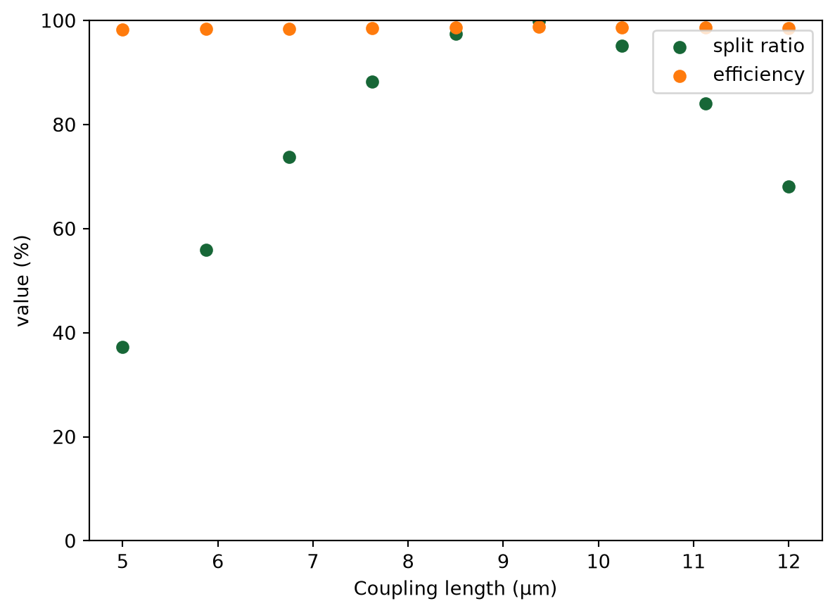
1D Parameter Scan#
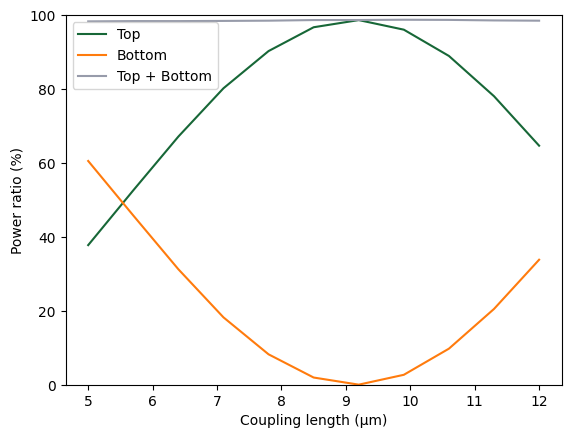
Now we will scan through the coupling length parameter to see the effect on splitting ratio.
To do this, we will create a list of simulations corresponding to each parameter combination.
We will use this list to create a Batch object, which has similar functionality to Job but allows one to manage a set of jobs.
First, we create arrays to store the input and output values.
[11]:
# create variables to store parameters, simulation information, results
Nl = 11

ls = np.linspace(5, 12, Nl)
split_ratios = np.zeros(Nl)
efficiencies = np.zeros(Nl)
Create Batch#
We now create our list of simulations and use them to initialize a Batch.
For more information, refer to the API reference.
[12]:
# submit all jobs
sims = {f"l={l:.2f}": make_sim(l, wg_spacing_coup) for l in ls}
batch = web.Batch(simulations=sims, verbose=True)
Monitor Batch#
Here we can perform real-time monitoring of how many of the jobs in the batch have completed.
[13]:
batch_results = batch.run(path_dir="data")
07:54:45 UTC Started working on Batch containing 11 tasks.
07:54:55 UTC Maximum FlexCredit cost: 6.246 for the whole batch.
             Use 'Batch.real_cost()' to get the billed FlexCredit cost after
             completion.
07:56:30 UTC Batch complete.
Load and Visualize Results#
Finally, we can compute the output quantities and load them into the arrays we created initially.
Then we may plot the results.
[14]:
amps_batch = []
for task_name, sim_data in batch_results.items():
    amps_arms_i = np.array(measure_transmission(sim_data))
    amps_batch.append(amps_arms_i)
amps_batch = np.stack(amps_batch, axis=1)
print(amps_batch.shape)  # (4, Nl)
print(amps_batch)
(4, 11)
[[-7.96867103e-03+1.46579921e-03j -9.56416251e-04-5.91058963e-03j
  -8.68835988e-03-2.71162438e-04j -2.74225304e-03+2.50200177e-03j
  -8.94530787e-03-9.62373517e-03j -1.79796694e-03+1.75609109e-03j
  -2.77898540e-03-9.46655009e-04j -8.61402199e-03-2.05064263e-03j
   6.85904075e-04-1.72143394e-03j -8.82217613e-03+1.86272084e-03j
  -1.55366664e-03-2.99435900e-03j]
 [ 7.08971446e-03-2.44072327e-03j -3.33912870e-03+4.29917985e-03j
   1.57092194e-03+3.25293574e-04j  9.30303498e-04-5.82406030e-05j
   4.44191243e-03+7.66279816e-03j -4.17260846e-03-2.07154260e-03j
   1.56630067e-03+5.48542022e-03j  4.22080704e-03+5.24719447e-05j
  -5.39943217e-03+3.84008287e-04j  5.56391684e-03+5.16260631e-03j
  -4.00964175e-03-1.00498435e-03j]
 [ 4.36866489e-01+4.18813924e-01j  6.68016138e-01-2.58010363e-01j
   2.43480647e-02-8.10820347e-01j -8.09735567e-01-3.65451949e-01j
  -6.94528272e-01+6.40745170e-01j  3.34775807e-01+9.21931962e-01j
   9.92136004e-01+5.04360256e-02j  4.45726295e-01-8.76566432e-01j
  -6.11497703e-01-7.27598692e-01j -8.57048874e-01+2.58498691e-01j
  -8.05838565e-02+8.15294114e-01j]
 [ 5.45800729e-01-5.64622460e-01j -2.45198390e-01-6.41230791e-01j
  -5.70536587e-01-1.94683812e-02j -1.83299921e-01+4.01908221e-01j
   2.05053806e-01+2.24036117e-01j  1.48048786e-01-5.34866699e-02j
   3.71450054e-04-7.10468822e-03j  1.27376809e-01+6.48012722e-02j
   2.21791540e-01-1.86578949e-01j -1.24771529e-01-4.11202761e-01j
  -5.57838782e-01-5.37826286e-02j]]
[15]:
powers = abs(amps_batch) ** 2
power_top = powers[2]
power_bot = powers[3]
power_out = power_top + power_bot
[16]:
plt.plot(ls, 100 * power_top, label="Top")
plt.plot(ls, 100 * power_bot, label="Bottom")
plt.plot(ls, 100 * power_out, label="Top + Bottom")
plt.xlabel("Coupling length (µm)")
plt.ylabel("Power ratio (%)")
plt.ylim(0, 100)
plt.legend()
plt.show()
Final Remarks#
Batches provide some other convenient functionality for managing large numbers of jobs.
For example, one can save the batch information to file and load the batch at a later time, if needing to disconnect from the service while the jobs are running.
[17]:
# save batch metadata
batch.to_file("data/batch_data.json")

# load batch metadata into a new batch
loaded_batch = web.Batch.from_file("data/batch_data.json")
For more reference, refer to our documentation.
Using the design Plugin#
In Tidy3D version 2.6.0, we introduced a Design plugin, which allows users to programmatically define and run their parameter scans while also providing a convenient container for managing the resulting data.
For more details, please refer to our full tutorial on the Design plugin.
We import the plugin through tidy3d.plugins.design below.
[18]:
import tidy3d.plugins.design as tdd
Then we define our sweep dimensions as tdd.ParameterFloat instances and give them each a range.
Note: we need to ensure that the
namearguments match the function argument names in ourmake_sim()function, which we will use to construct the simulations for the parameter scan.
[19]:
param_spc = tdd.ParameterFloat(name="wg_spacing_coup", span=(0.1, 0.15), num_points=3)
param_len = tdd.ParameterFloat(name="coup_length", span=(5, 12), num_points=3)
For this example, we will do a grid search over these points, which we can define a tdd.MethodGrid and then combine everything into a tdd.DesignSpace.
[20]:
method = tdd.MethodGrid()
design_space = tdd.DesignSpace(
    parameters=[param_spc, param_len],
    method=method,
    task_name="ParameterScan_Notebook",
    path_dir="./data",
)
To run the sweep, we need to pass the design space our evaluation function. Here we will define it through pre and post processing functions, which enables the design plugin to take advantage of parallelism to perform Batch processing under the hood.
The functions make_sim and measure_transmission already almost work perfectly as pre and post processing functions. We’ll just wrap measure_transmission to return a dictionary of the amplitudes, so that the dictionary keys can be used to label the outputs in the resulting dataset.
[21]:
def fn_post(*args, **kwargs):
    """Post processing function, but label the outputs using a dictionary."""
    a, b, c, d = measure_transmission(*args, **kwargs)
    return dict(input=a, reflect_bottom=b, top=c, bottom=d)
Finally, we pass our pre-processing and post-processing functions to the DesignSpace.run_batch() method to get our results.
[22]:
results = design_space.run(fn=make_sim, fn_post=fn_post)
07:56:35 UTC Running 9 Simulations
Let’s get a pandas.DataFrame of the results and print out the first 5 elements.
[23]:
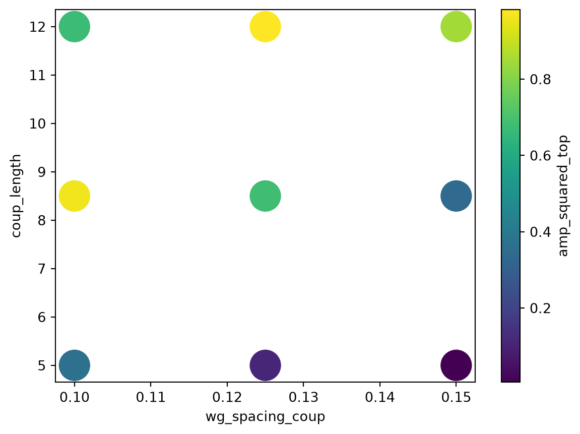
df = results.to_dataframe()

# take absolute value squared of output 2 to get powers to the top port
df["amp_squared_top"] = df["top"].map(lambda x: abs(x) ** 2)

df.head()