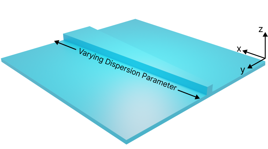
Tapered Waveguide#

The tapered waveguide is 5 mm long and varies adiabatically from 0.500 $\mu m$ to 1.100 $\mu m$ in width. The rib cross-section has a total height of 0.380 $\mu m$ and a slab thickness of 0.065 $\mu m$. The waveguide is etched into a silicon thin film and is surrounded by a thick silica layer.

[2]:

taper_w_in = 0.5  # Input taper width (um).
taper_w_out = 1.1  # Output taper width (um).
taper_l = 5000  # Taper length (um).
wg_h = 0.38  # Waveguide height (um).
wg_slab = 0.065  # Waveguide slab thickness (um).

The group-velocity dispersion (GVD) variation will be computed along the taper length at the wavelength of 1.95 $\mu m$. In addition, we will calculate the dispersion parameter (D) between the wavelength range of 1.2 $\mu m$ and 2.8 $\mu m$.

[3]:

wl_min = 1.2  # Minimum wavelength in dispersion calculation.
wl_max = 2.4  # Maximum wavelength in dispersion calculation.
wl_steps = 21  # Number of wavelength points in mode calculation.

wl_d = np.linspace(wl_min, wl_max, wl_steps)  # Wavelength range for D calculation.
wl_gvd = np.asarray([1.95])  # Wavelength for GVD calculation.

Simulation Setup#

Now, we will build the tapered waveguide structure using a `PolySlab <https://docs.flexcompute.com/projects/tidy3d/en/latest/api/_autosummary/tidy3d.PolySlab.html>`__ and materials taken from the material library.

[4]:

mat_si = td.material_library["cSi"]["Palik_Lossless"]
mat_sio2 = td.material_library["SiO2"]["Palik_Lossless"]

taper = td.Structure(
    geometry=td.PolySlab(
        vertices=[
            [0, -taper_w_in / 2],
            [taper_l, -taper_w_out / 2],
            [taper_l, taper_w_out / 2],
            [0, taper_w_in / 2],
        ],
        axis=2,
        slab_bounds=(-wg_h / 2, wg_h / 2),
    ),
    medium=mat_si,
    name="taper_core",
)

slab = td.Structure(
    geometry=td.Box(center=[0, 0, -wg_h / 2 + wg_slab / 2], size=[td.inf, td.inf, wg_slab]),
    medium=mat_si,
    name="taper_slab",
)

sim = td.Simulation(
    center=(taper_l / 2, 0, 0),
    size=(1.1 * taper_l, taper_w_out + wl_max, 3),
    grid_spec=td.GridSpec.auto(min_steps_per_wvl=15, wavelength=wl_min),
    structures=[taper, slab],
    run_time=1e-12,
    medium=mat_sio2,
    boundary_spec=td.BoundarySpec.all_sides(boundary=td.Periodic()),
    symmetry=(0, -1, 0),
)

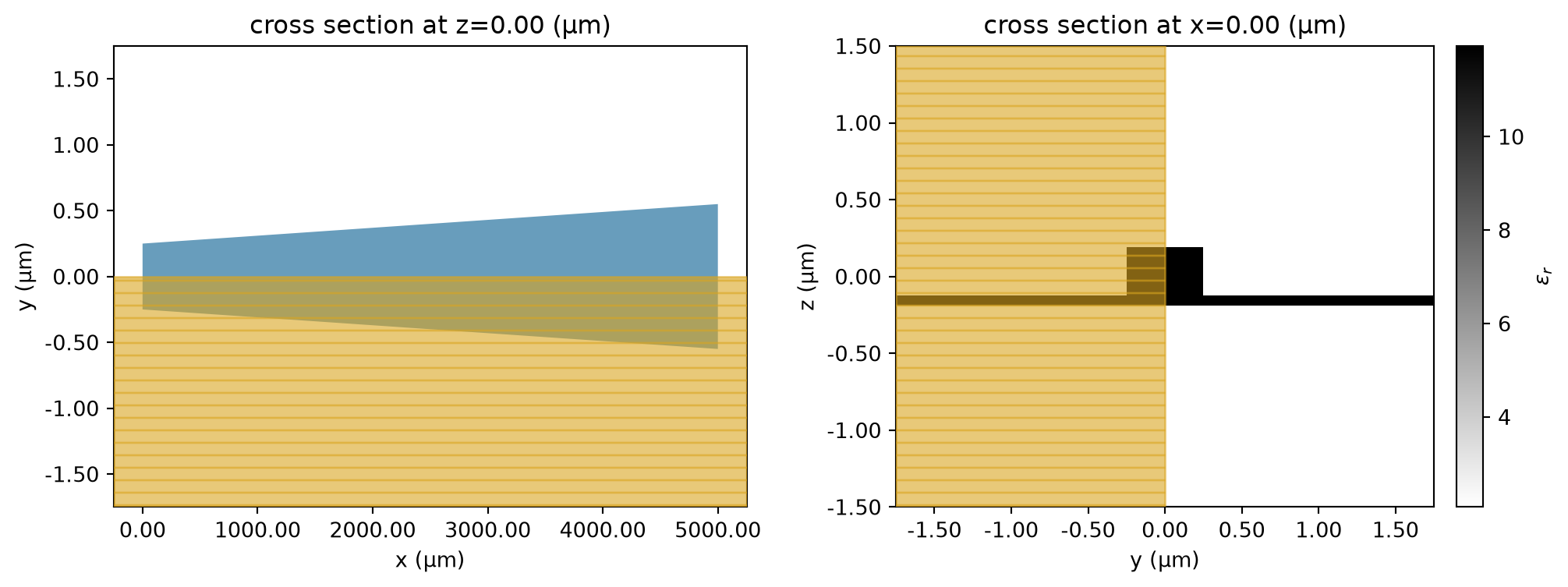
To ensure the simulation is correctly defined, we will visualize the permittivity distribution. As expected, we see the tapered waveguide profile along the x-direction and the rib cross-section in the yz plane.

[5]:

fig, ax = plt.subplots(1, 2, figsize=(12, 4))
sim.plot(z=0, ax=ax[0])
ax[0].set_aspect("auto")

sim.plot_eps(x=0, freq=td.C_0 / wl_gvd[0], ax=ax[1])
plt.show()

As we need to run the mode solver several times, we will create a helper function called build_mode. This function takes the arguments mode_pos_x, wl, num_modes, and group_index_step, and builds the ModeSolver. We plan to use this function to conduct a sweep on the mode plane position along the tapered waveguide to calculate the parameters D and GVD.

[6]:

def build_mode(
    mode_pos_x: float = 0, wl: np.array = wl_d, num_modes: int = 1, group_index_step: float = 0.15
) -> ModeSolver:
    """Builds a ModeSolver object."""

    freqs = td.C_0 / wl  # Mode frequencies.

    # Mode specification.
    mode_spec = td.ModeSpec(
        num_modes=num_modes,
        group_index_step=group_index_step,
        num_pml=[7, 7],
    )

    # Build a mode solver.
    mode_solver = ModeSolver(
        simulation=sim,
        plane=td.Box(center=(mode_pos_x, 0, 0), size=(0, td.inf, td.inf)),
        mode_spec=mode_spec,
        freqs=freqs,
    )

    return mode_solver

Group Index Step Convergence#

According to [2] G. Agrawal. Nonlinear Fiber Optics (5th Ed.), Academic Press (2013), the effects of fiber dispersion are addressed by expanding the mode-propagation constant $\beta$ in a Taylor series around the angular frequency $\omega$. As a result, the parameters ${\beta }_1$ and ${\beta }_2$ are directly linked to the mode’s effective index $n_{eff}(\omega )$ and its derivatives as

and

where $c$ is the speed of light, $v_g$ is the group velocity, and $n_g$ is the group index. The first-order term ${\beta }_1$ controls the speed at which the optical pulse envelope propagates, and the group velocity dispersion (GVD) parameter ${\beta }_2$ represents dispersion of the group velocity and is responsible for pulse broadening. In practice, the dispersion parameter D, which is defined as $d{\beta }_1/d\lambda$, is also used to quantify dispersion. It is related to ${\beta }_2$ by

where $\lambda$ is the light wavelength.

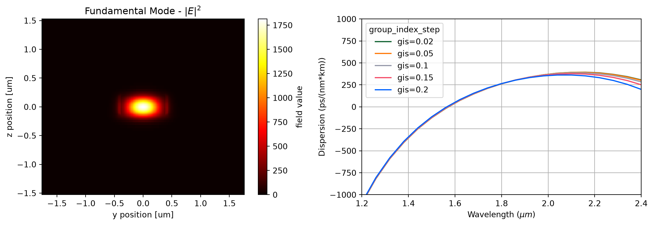
When calculating dispersion using the Tidy3D ModeSolver, additional frequency points are included to improve the accuracy of the effective index numerical differentiation. The parameter group_index_step controls the proximity of these additional frequency points to the user-supplied frequencies. Before proceeding with the main analyses, we will verify the convergence of our dispersion calculation with respect to the group_index_step parameter.

We will build a dictionary of ModeSolver instances to create a simulation batch as we run many mode solver calculations.

[7]:

# List of group_index_step values.
gis_values = [0.02, 0.05, 0.10, 0.15, 0.20]

# Mode sweep over the group_index_step values.
mode_gis = {}
for gis in gis_values:
    mode_gis[f"gis={gis}"] = build_mode(mode_pos_x=taper_l / 2, group_index_step=gis)

Once the batch of ModeSolvers is created, we simply use the run() method to run the entire batch of tasks in parallel.

[8]:

#  Run the mode solvers in parallel.
batch = web.Batch(simulations=mode_gis)
batch_gis = batch.run(path_dir="data")

16:25:19 Eastern Standard Time Started working on Batch containing 5 tasks.

16:25:22 Eastern Standard Time Maximum FlexCredit cost: 0.029 for the whole
                               batch.

                               Use 'Batch.real_cost()' to get the billed
                               FlexCredit cost after the Batch has completed.

16:25:24 Eastern Standard Time Batch complete.

We can observe that a group_index_step value between 0.10 and 0.15 is enough to obtain a smooth dispersion curve, avoiding the numerical noise created in smaller group_index_step values.

[9]:

fig, ax = plt.subplots(1, 2, figsize=(12, 4), tight_layout=True)

batch_gis[f"gis={gis_values[0]}"].intensity.isel(
    f=batch_gis[f"gis={gis_values[0]}"].modes_info["f"].size // 2, mode_index=0
).plot(x="y", y="z", cmap="hot", ax=ax[0])
ax[0].set_title("Fundamental Mode - $|E|^{2}$")
ax[0].set_aspect("equal")

for gis, md in batch_gis.items():
    ax[1].plot(
        td.C_0 / md.modes_info["f"].squeeze(drop=True).values,
        md.modes_info["dispersion (ps/(nm km))"].squeeze(drop=True).values,
        label=gis,
    )
ax[1].set_ylabel("Dispersion (ps/(nm*km))")
ax[1].set_xlabel("Wavelength ($\\mu m$)")
ax[1].set_ylim([-1000, 1000])
ax[1].set_xlim([wl_d[0], wl_d[-1]])
ax[1].legend(title="group_index_step")
ax[1].grid()
plt.show()

Dispersion Parameters Calculation#

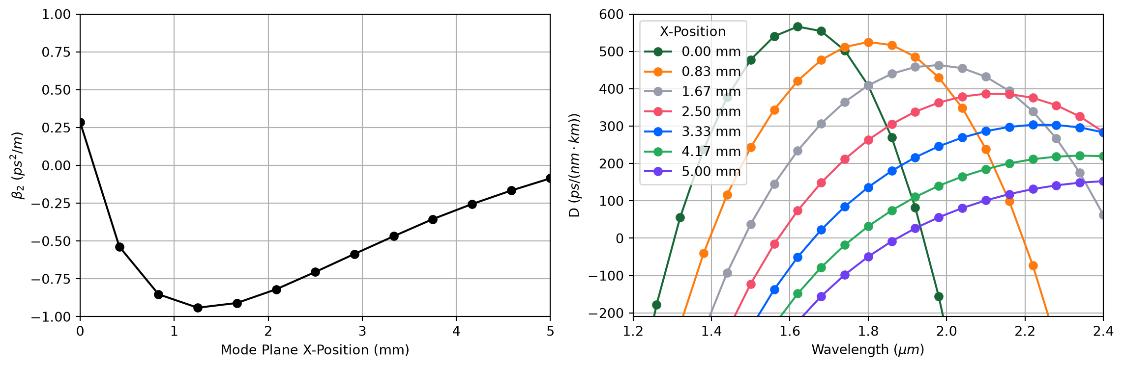
Now, we are ready to calculate the dispersion parameters for the varying waveguide cross-sections along the taper length. To reproduce Figure 5(a) of [1], we will calculate the ${\beta }_2$ parameter of GVD at the wavelength of 1.95 $\mu m$ for waveguide cross-sections ranging from 0.5 $\mu m$ to 1.1 $\mu m$ in intervals of 0.2 $\mu m$.

[10]:

x_values_gvd = np.linspace(0.05, taper_l - 0.05, 13)

# Mode simulations to calculate beta2 of GVD.
mode_gvd = {}
for x in x_values_gvd:
    mode_gvd[f"x={x:.2f}"] = build_mode(mode_pos_x=x, wl=wl_gvd, group_index_step=0.15)

[11]:

#  Run the mode solvers in parallel.
batch = web.Batch(simulations=mode_gvd)
batch_gvd = batch.run(path_dir="data")

16:25:42 Eastern Standard Time Started working on Batch containing 13 tasks.

16:25:52 Eastern Standard Time Maximum FlexCredit cost: 0.048 for the whole
                               batch.

                               Use 'Batch.real_cost()' to get the billed
                               FlexCredit cost after the Batch has completed.

16:25:58 Eastern Standard Time Batch complete.

[12]:

# Mode simulations to calculate beta2 of GVD.
data_gvd = []
for _, md in batch_gvd.items():
    d = md.modes_info["dispersion (ps/(nm km))"].squeeze(drop=True).values
    beta2 = -((d * wl_gvd**2) / (2 * np.pi * td.C_0)) * 1e12
    data_gvd.append(beta2)

Afterward, considering seven positions along the taper length, we will calculate the dispersion parameter D for wavelengths ranging from 1.2 $\mu m$ to 2.4 $\mu m$. We will use this data to plot Figure 5(b) of [1].

[13]:

x_values_d = np.linspace(0.05, taper_l - 0.05, 7)

# Mode simulations to calculate D.
mode_d = {}
for x in x_values_d:
    mode_d[f"x={x:.2f}"] = build_mode(mode_pos_x=x, group_index_step=0.1)

[14]:

#  Run the mode solvers in parallel.
batch = web.Batch(simulations=mode_d)
batch_d = batch.run(path_dir="data")

16:26:15 Eastern Standard Time Started working on Batch containing 7 tasks.

16:26:20 Eastern Standard Time Maximum FlexCredit cost: 0.041 for the whole
                               batch.

                               Use 'Batch.real_cost()' to get the billed
                               FlexCredit cost after the Batch has completed.

16:26:23 Eastern Standard Time Batch complete.

[15]:

data_d = []
for _, md in batch_d.items():
    data_d.append(md.modes_info["dispersion (ps/(nm km))"].squeeze(drop=True).values)

Lastly, we will plot GVD and D dispersion parameters. We can observe a good agreement between the simulations and Figure 5(a-b).

[16]:

fig, ax = plt.subplots(1, 2, figsize=(12, 4), tight_layout=True)

# GVD
ax[0].plot(x_values_gvd / 1000, data_gvd, "ok-")
ax[0].set_ylabel("$\\beta_{2}$ ($ps^{2}/m$)")
ax[0].set_xlabel("Mode Plane X-Position (mm)")
ax[0].set_ylim([-1, 1])
ax[0].set_xlim([0, 5])
ax[0].grid()

# D
for l, d in zip(x_values_d, data_d):
    ax[1].plot(wl_d, d, "-o", label=f"{l /1000:.2f} mm")
ax[1].set_ylabel("D ($ps/(nm \\cdot km)$)")
ax[1].set_xlabel("Wavelength ($\\mu m$)")
ax[1].set_ylim([-210, 600])
ax[1].set_xlim([1.2, 2.4])
ax[1].legend(title="X-Position")
ax[1].grid()
plt.show()

[ ]: