Extracting resonance information using Resonance Finder#
When looking for long-lived resonances using FDTD simulation, the total time to fully decay fields within the simulation domain can be extremely long. In this situation, the Resonance Finder plugin allows one to find resonances and extract their information from time domain field monitors without the necessity of waiting for the fields to completely decay. The resonance information consisting of frequency \(f\), decay rate \(\alpha\), Q-factor, amplitude \(a\), and phase \(\phi\) is obtained from a time series of the form:
where \(k\) is the frequency of interest index. The resonance finder algorithm was derived from V. A. Mandelshtam, and H. S. Taylor, “Harmonic inversion of time signals and its applications,” J. Chem. Phys. 107(17), 6756–6769 (1997), DOI: 10.1063/1.475324. This notebook illustrates the tool usage through the example of a simple photonic cavity. More examples on using the resonance finder in different applications are available in Optimized photonic crystal L3 cavity, Band structure calculation of a photonic crystal slab, or Bistability in photonic crystal microcavities notebooks.
If you are new to the finite-difference time-domain (FDTD) method, we highly recommend going through our FDTD101 tutorials. FDTD simulations can diverge due to various reasons. If you run into any simulation divergence issues, please follow the steps outlined in our troubleshooting guide to resolve it.
To start, we need to import the Tidy3D resonance finder plugin as below:
[1]:
# Standard python imports.
import matplotlib.pyplot as plt
import numpy as np

# Tidy3D imports.
import tidy3d as td
import tidy3d.web as web
from tidy3d.plugins.resonance import ResonanceFinder
Microdisk Cavity Set Up#
To illustrate the resonance finder usage, we will define a simple GaAs microdisk cavity.
[2]:
# Simulation wavelength
wl_min = 1.9
wl_max = 2.0
n_wl = 101
wl_c = (wl_min + wl_max) / 2
wl_range = np.linspace(wl_min, wl_max, n_wl)
freq_c = td.C_0 / wl_c
freq_range = td.C_0 / wl_range
freq_bw = 0.5 * (freq_range[0] - freq_range[-1])

# Simulation runtime
runtime_fwidth = 20  # In units of 1/frequency bandwidth of the source.
t_start_fwidth = (
    2  # Time to start monitoring after source has decayed, units of 1/frequency bandwidth.
)
run_time = runtime_fwidth / freq_bw
t_start = t_start_fwidth / freq_bw
print(f"Total runtime = {(run_time * 1e12):.2f} ps")
print(f"Start monitoring fields after {(t_start * 1e12):.2f} ps")

# Microdisk geometry
r = 2.60
t = 0.16

# Microdisk material
n = 3.50
mat_disk = td.Medium(permittivity=n**2)
Total runtime = 5.07 ps
Start monitoring fields after 0.51 ps
The microdisk structure is obtained using a simple cylinder.
[3]:
# Simulation size.
pml_gap = 0.6 * wl_max
size_x = 2 * (r + pml_gap)
size_y = size_x
size_z = t + 2 * pml_gap

# Microdisk.
microdisk = td.Structure(
    geometry=td.Cylinder(center=(0, 0, 0), radius=r, length=t, axis=2),
    medium=mat_disk,
)
We will use several point dipole sources randomly distributed within a squared region bounded by the microdisk to excite the cavity modes. Reproducibility between simulation runs is ensured by seeding the random generator. We limit the dipole polarizations to only one direction as we will include 8-fold symmetry.
[4]:
num_dipoles = 7
rng = np.random.default_rng(4321)

# Squared region within microdisk.
side_x = r * np.cos(45 * np.pi / 180)
side_y = r * np.cos(45 * np.pi / 180)

# Build random positions and phases to dipoles.
dip_positions = rng.uniform([0, 0, 0], [side_x, side_y, 0], [num_dipoles, 3])
dip_phases = rng.uniform(0, 2 * np.pi, num_dipoles)

# Dipoles
pulses = []
dipoles = []
for i in range(num_dipoles):
    pulse = td.GaussianPulse(freq0=freq_c, fwidth=freq_bw, phase=dip_phases[i])
    pulses.append(pulse)
    dipoles.append(
        td.PointDipole(
            source_time=pulse,
            center=tuple(dip_positions[i]),
            polarization="Ey",
            name="dip_source_" + str(i),
        )
    )
The Resonance Finder plugin needs FieldTimeMonitors to record the field as a function of time. So, we will include them at several random locations. Importantly, we start the monitors after the source pulse has decayed.
[5]:
num_monitors = 7

# Random monitor positions.
mon_positions = rng.uniform([0, 0, 0], [side_x, side_y, 0], [num_dipoles, 3])

# Monitor list.
monitors_time = []
for i in range(num_monitors):
    monitors_time.append(
        td.FieldTimeMonitor(
            fields=["Ey"],
            center=tuple(mon_positions[i]),
            size=(0, 0, 0),
            start=t_start,
            name="monitor_time_" + str(i),
        )
    )
Microdisk Cavity Simulation#
Now, we can build and run the simulation. It is worth mentioning that we will run the simulation for a shorter run_time period, thus not waiting a very long time for the fields to decay fully.
Note on symmetry: In this example, we use symmetry=(1, -1, 1) to take advantage of the microdisk’s geometric symmetry and reduce the computation cost. However, it is important to be aware that applying symmetry constraints means that only modes whose field profiles are compatible with the specified symmetry will be excited and detected by the resonance finder. Modes with different symmetry properties (e.g., modes that are anti-symmetric where a symmetric boundary condition is enforced,
or vice versa) will be filtered out and will not appear in the results. If you need to find all supported modes of a structure, consider either removing the symmetry setting or running multiple simulations with different symmetry combinations to capture modes of all symmetry classes.
For more background, see the symmetry tutorial.
[6]:
sim = td.Simulation(
    center=(0, 0, 0),
    size=(size_x, size_y, size_z),
    grid_spec=td.GridSpec.auto(min_steps_per_wvl=20, wavelength=wl_c),
    structures=[microdisk],
    sources=dipoles,
    monitors=monitors_time,
    run_time=run_time,
    shutoff=0,
    boundary_spec=td.BoundarySpec.all_sides(boundary=td.PML()),
    normalize_index=None,
    symmetry=(1, -1, 1),
)

sim.plot_3d(width=400, height=400)
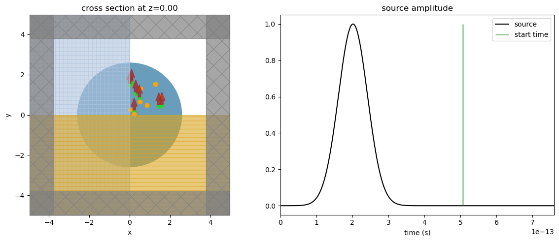
Before running the simulation, let’s look at the source and monitor positions and certify we are measuring the fields after the sources have fully decayed.
[7]:
fig, (ax1, ax2) = plt.subplots(1, 2, tight_layout=True, figsize=(12, 5))
sim.plot(z=0.0, ax=ax1)

plot_time = 3 / freq_bw
sim.sources[0].source_time.plot(times=np.linspace(0, plot_time, 1001), val="abs", ax=ax2)
ax2.set_xlim(0, plot_time)
ax2.vlines(t_start, 0, 1, linewidth=2, color="g", alpha=0.4)
ax2.legend(["source", "start time"])
plt.show()
[8]:
job = web.Job(simulation=sim, task_name="microdisk", verbose=False)
sim_data = job.run(path="data/simulation_data.hdf5")
Cavity Resonance Information#
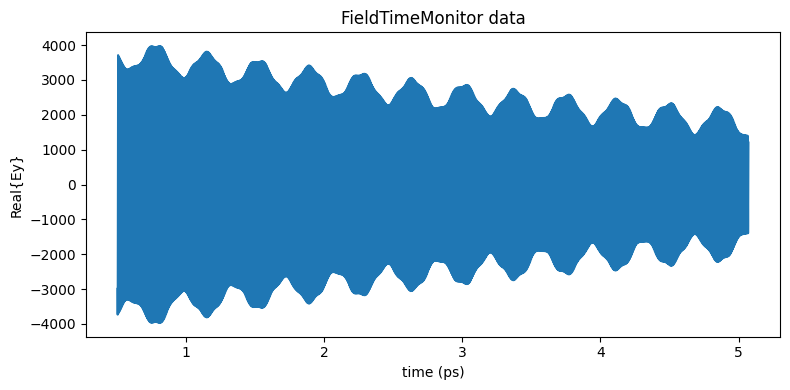
Now, we can analyze the simulation data and calculate the resonance information from the time domain fields. First, let’s look at one of the FieldTimeMonitors data. As expected, it is clear from the source signal, and a decaying oscillating pattern due to the cavity resonances is shown.
[9]:
fig, ax1 = plt.subplots(1, 1, tight_layout=True, figsize=(8, 4))

ax1.plot(
    sim_data.monitor_data["monitor_time_0"].Ey.t * 1e12,
    np.real(sim_data.monitor_data["monitor_time_0"].Ey.squeeze()),
)
ax1.set_title("FieldTimeMonitor data")
ax1.set_xlabel("time (ps)")
ax1.set_ylabel("Real{Ey}")
plt.show()
We first construct a ResonanceFinder object storing our parameters and then call run() on our list of FieldTimeData objects. This will add up the signals from all monitors before searching for resonances. Additionally, the ResonanceFinder class has the methods run_raw_signal and
run_scalar_field_time which are helpful case the signal takes another form.
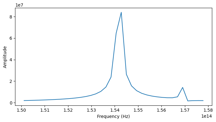
The run() method returns an xr.Dataset containing the decay rate, Q factor, amplitude, phase, and estimation error for each resonance as a function of frequency.
[10]:
resonance_finder = ResonanceFinder(freq_window=(freq_range[-1], freq_range[0]))
resonance_data = resonance_finder.run(signals=sim_data.data)
resonance_data.to_dataframe()