Biosensor grating simulation#
Bragg gratings are structures that involve a periodic variation in the refractive index or geometry of waveguide, so that certain frequencies of light are reflected off the grating while others are transmitted.
Since gratings can be designed to be extremely sensitive, one possible application they have is to detect the presence of foreign molecules. If particles such as biomolecules are deposited on the device, it will no longer have the same reflective properties in the band of frequencies for which it was designed. Therefore, carefully designed Bragg gratings can be used as biosensors.
In this example, an optical biosensor grating is modeled to detect the presence of biomolecules. The grating is designed to be reflective over a narrow band around its resonant frequency, which is modified by the presence of a biomolecule.
Reference: Brian Cunningham, Bo Lin, Jean Qiu, Peter Li, Jane Pepper, Brenda Hugh, "A plastic colorimetric resonant optical biosensor for multiparallel detection of label-free biochemical interactions," Sensors and Actuators B 85 (2002), DOI: 10.1016/S0925-4005(02)00111-9.
If you are new to the finite-difference time-domain (FDTD) method, we highly recommend going through our FDTD101 tutorials.
[1]:
# basic imports
import matplotlib.pylab as plt
import numpy as np

# Tidy3D imports
import tidy3d as td
Structure Setup#
Create the grating geometry.
[2]:
# materials
Si3N4 = td.Medium(permittivity=2.05**2)
epoxy = td.Medium(permittivity=1.5**2)
background = td.Medium(permittivity=1.333**2)

# set basic geometric parameters (units in microns)
nm = 1e-3
period = 550 * nm
grating_fill_factor = 0.5
grating_height = 200 * nm
film_height = 120 * nm
epoxy_height = 380 * nm
monitor_distance = 1.0
monitor_gap = 0.1

# the epoxy layer top surface is at z=0
sim_center = (0, 0, 0.5 * (grating_height + film_height - epoxy_height))
sim_size = (
    period,
    0,
    epoxy_height + grating_height + film_height + 2 * (monitor_distance + monitor_gap),
)

# wavelength / frequency setup
wavelength_min = 770 * nm
wavelength_max = 900 * nm
freq_min = td.C_0 / wavelength_max
freq_max = td.C_0 / wavelength_min
freq0 = (freq_min + freq_max) / 2.0
fwidth = freq_max - freq_min
run_time = 10e-12

# epoxy layer
epoxy_layer = td.Structure(
    geometry=td.Box(
        center=[0.0, 0.0, -0.5 * epoxy_height],
        size=[td.inf, td.inf, epoxy_height],
    ),
    medium=epoxy,
    name="epoxy_layer",
)

# bottom Si3N4 film layer
bottom_film = td.Structure(
    geometry=td.Box(
        center=[0.0, 0.0, 0.5 * film_height],
        size=[td.inf, td.inf, film_height],
    ),
    medium=Si3N4,
    name="bottom_film",
)

# epoxy grating teeth (partially covers the film layer)
grating_teeth = td.Structure(
    geometry=td.Box(
        center=[0.0, 0.0, 0.5 * grating_height],
        size=[period * grating_fill_factor, td.inf, grating_height],
    ),
    medium=epoxy,
    name="grating_teeth",
)

# top Si3N4 film layer
top_film = td.Structure(
    geometry=td.Box(
        center=[0.0, 0.0, grating_height + 0.5 * film_height],
        size=[period * grating_fill_factor, td.inf, film_height],
    ),
    medium=Si3N4,
    name="top_film",
)

# the order her matters, because the teeth must override the bottom film layer
geometry = [epoxy_layer, bottom_film, grating_teeth, top_film]

# boundary conditions: the simulation is periodic in the x-y plane, and simulates
# an infinite domain along z
boundary_spec = td.BoundarySpec(
    x=td.Boundary.periodic(),
    y=td.Boundary.periodic(),
    z=td.Boundary.pml(),
)

# grid specification
grid_spec = td.GridSpec.auto(min_steps_per_wvl=30)
Source Setup#
Create the plane wave source which excites the structure from underneath.
[3]:
source_time = td.GaussianPulse(freq0=freq0, fwidth=fwidth)
source = td.PlaneWave(
    center=[0, 0, -(epoxy_height + monitor_distance - monitor_gap)],
    size=[td.inf, td.inf, 0.0],
    source_time=source_time,
    pol_angle=0,
    direction="+",
)
Monitor Setup#
Create field and flux monitors to measure reflecting and transmitted flux.
[4]:
# create field monitor
monitor_xz = td.FieldMonitor(
    center=sim_center,
    size=[td.inf, 0, td.inf],
    freqs=[freq0],
    name="fields_xz",
)

# create flux monitors
freqs = np.linspace(freq_min, freq_max, 1000)
monitor_flux_refl = td.FluxMonitor(
    center=[0, 0, -(epoxy_height + monitor_distance)],
    size=[td.inf, td.inf, 0.0],
    freqs=freqs,
    name="flux_refl",
)
monitor_flux_tran = td.FluxMonitor(
    center=[0, 0, grating_height + film_height + monitor_distance],
    size=[td.inf, td.inf, 0.0],
    freqs=freqs,
    name="flux_tran",
)

monitors = [monitor_xz, monitor_flux_refl, monitor_flux_tran]
Create Simulation#
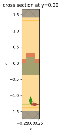
The final simulation object is created and visualized.
[5]:
# create the simulation
sim = td.Simulation(
    center=sim_center,
    size=sim_size,
    grid_spec=grid_spec,
    structures=geometry,
    sources=[source],
    monitors=monitors,
    run_time=run_time,
    boundary_spec=boundary_spec,
    medium=background,
    shutoff=1e-6,
)

# plot the simulation domain
sim.plot(y=0)
plt.show()
Run Simulation#
[6]:
# run simulation
import tidy3d.web as web

sim_data = web.run(sim, task_name="biosensor", path="data/biosensor.hdf5", verbose=True)
19:24:03 CEST Created task 'biosensor' with task_id
              'fdve-8c36c09e-e802-4d0e-b920-4fd13a70d138' and task_type 'FDTD'.
              View task using web UI at
              'https://tidy3d.simulation.cloud/workbench?taskId=fdve-8c36c09e-e8
              02-4d0e-b920-4fd13a70d138'.
Task folder: 'default'.
19:24:04 CEST Maximum FlexCredit cost: 0.025. Minimum cost depends on task
              execution details. Use 'web.real_cost(task_id)' to get the billed
              FlexCredit cost after a simulation run.
19:24:05 CEST status = queued
              To cancel the simulation, use 'web.abort(task_id)' or
              'web.delete(task_id)' or abort/delete the task in the web UI.
              Terminating the Python script will not stop the job running on the
              cloud.
19:27:15 CEST status = preprocess
19:27:20 CEST starting up solver
running solver
19:27:31 CEST early shutoff detected at 32%, exiting.
status = success
              View simulation result at
              'https://tidy3d.simulation.cloud/workbench?taskId=fdve-8c36c09e-e8
              02-4d0e-b920-4fd13a70d138'.
19:27:33 CEST loading simulation from data/biosensor.hdf5
Plot Fields#
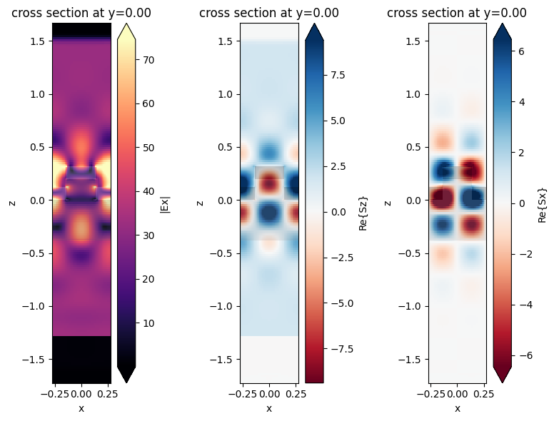
The frequency-domain fields recorded are plotted at the center frequency in an xz plane. The resonance can be clearly seen in the power flow pattern shown by the Poynting vector plots.
[7]:
fig, ax = plt.subplots(1, 3, figsize=(8, 6), tight_layout=True)

sim_data.plot_field("fields_xz", field_name="Ex", val="abs", f=freq0, ax=ax[0])
sim_data.plot_field("fields_xz", field_name="Sz", val="real", f=freq0, ax=ax[1])
sim_data.plot_field("fields_xz", field_name="Sx", val="real", f=freq0, ax=ax[2])
plt.show()
Plot Transmission and Reflection#
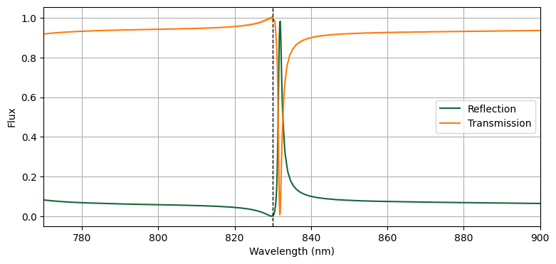
To see the effectiveness of the grating, we can compute and plot the reflection and transmission via the flux measured by the flux monitor. As the plot shows, the structure is highly reflective in a narrow frequency range around the design frequency, allowing one to detect small variations in the frequency response due to the presence of biological materials. The vertical dashed line shows the wavelength used in the previous plots.
[8]:
transmission = sim_data["flux_tran"].flux
reflection = -sim_data["flux_refl"].flux

fig, ax = plt.subplots(figsize=(9, 4))

ax.plot(td.C_0 / freqs * 1e3, reflection, label="Reflection")
ax.plot(td.C_0 / freqs * 1e3, transmission, label="Transmission")

# wavelength for the field plots
ax.axvline(td.C_0 / freq0 * 1e3, ls="--", color="k", lw=1)

ax.set(
    xlabel="Wavelength (nm)",
    ylabel="Flux",
    xlim=(wavelength_min * 1e3, wavelength_max * 1e3),
)
ax.legend()
ax.grid()
plt.show()