Basics#

The Design plugin (tidy3d.plugins.design) is a user-friendly tool that simplifies the process of defining and optimizing experiments within the Tidy3D environment. This plugin helps you efficiently explore different design possibilities by setting up a structured approach to test and refine your ideas.

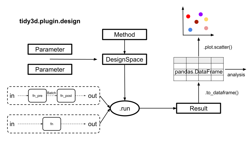
To get started, define the key Parameters of your design problem and choose a Method that will suggest possible solutions. The Method can sample the design space systematically or randomly using MethodGrid or MethodMonteCarlo, or can optimize for a given problem through iterative search and evaluation using techniques like Bayesian optimization (MethodBayOpt), genetic algorithm (MethodGenAlg) or particle swarm optimization (MethodParticleSwarm). These choices are combined into a DesignSpace object, which serves to manage the search process.

Next, provide a function that describes the relationship between your input variables (the dimensions of your design) and the desired outputs. This function can take any inputs and return any outputs that you want to investigate.

The results of the search are automatically stored in a Result object. This object contains all the details of the search and can be quickly converted into a pandas.DataFrame for further analysis, post-processing, or visualization. In this DataFrame, each column represents an input or output from your function, and each row represents a single data point from your experiment.

Here’s a diagram to details the process step-by-step.

Another example of the Design plugin can be seen about halfway down our Parameter Scan notebook. A simple practical case study of the Design plugin is available in the All-Dielectric Structural Color notebook, or more complex case studies in the following optimization notebooks:

1. Bayesian Optimization of Y-Junction

2. Particle Swarm Optimizer PBS

3. Particle Swarm Optimizer Bullseye Cavity

4. Genetic Algorithm Reflector

The plugin is imported from tidy3d.plugins.design so it’s convenient to import this namespace first along with the other packages we need.

[2]:

import numpy as np
import matplotlib.pylab as plt
import typing

import tidy3d as td
import tidy3d.plugins.design as tdd

Quickstart#

While the Design plugin is built for Tidy3D and has special features for handling FDTD simulations, it can also be run with any general design problem. Here is a quick, complete example before diving into the use of the plugin with Tidy3D simulations.

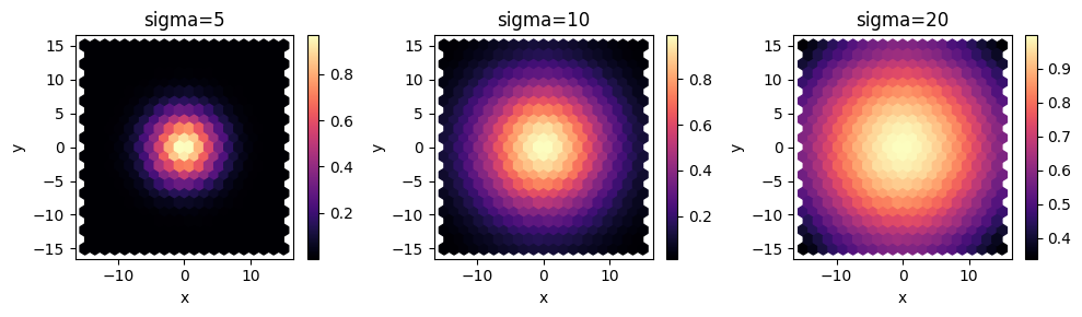
Here we want to sample a design space with two dimensions x and y with Monte Carlo. Our function simply returns a Gaussian centered at (0,0) and we’ll evaluate the result for Gaussians with 3 different variances.

[3]:

# Define your design space (parameters (x,y) within certain ranges)
param_x = tdd.ParameterFloat(name="x", span=(-15,15))
param_y = tdd.ParameterFloat(name="y", span=(-15,15))

# Define your sampling method, Monte Carlo method with 10,000 points
method = tdd.MethodMonteCarlo(num_points=10000)

# Put everything together in a `DesignSpace` container
design_space = tdd.DesignSpace(method=method, parameters=[param_x, param_y])

# Define your fitness function / figure of merit. Here we compute a gaussian as a function of x and y with different values for the width.
sigmas = {f"sigma={s}": s for s in [5, 10, 20]}
def f(x:float, y:float) -> typing.Dict[str, float]:
    """gaussian distribution as a function of x and y."""
    r2 = x**2 + y**2
    gaussian = lambda sigma: np.exp(-r2 / sigma ** 2)
    # return a dictionary, where the key is used to label the output names
    return {key: gaussian(sigma) for key, sigma in sigmas.items()}

# Call .run on the DesignSpace with our function and convert the results to a pandas.DataFrame
df = design_space.run(f).to_dataframe()

# Plot the results using pandas.DataFrame builtins
f, axes = plt.subplots(1, 3, figsize=(10, 3), tight_layout=True)
for ax, C in zip(axes, sigmas.keys()):
    _ = df.plot.hexbin(x='x', y='y', gridsize=20, C=C, cmap="magma", ax=ax)
    ax.set_title(C)

[4]:

# Look at the first 5 outputs
df.head()

[4]:

Design Space Exploration in Tidy3D#

We can repeat the same process to perform a parameter sweep of a photonic device. The only difference is that for our function evaluation each point will involve a Tidy3D Simulation.

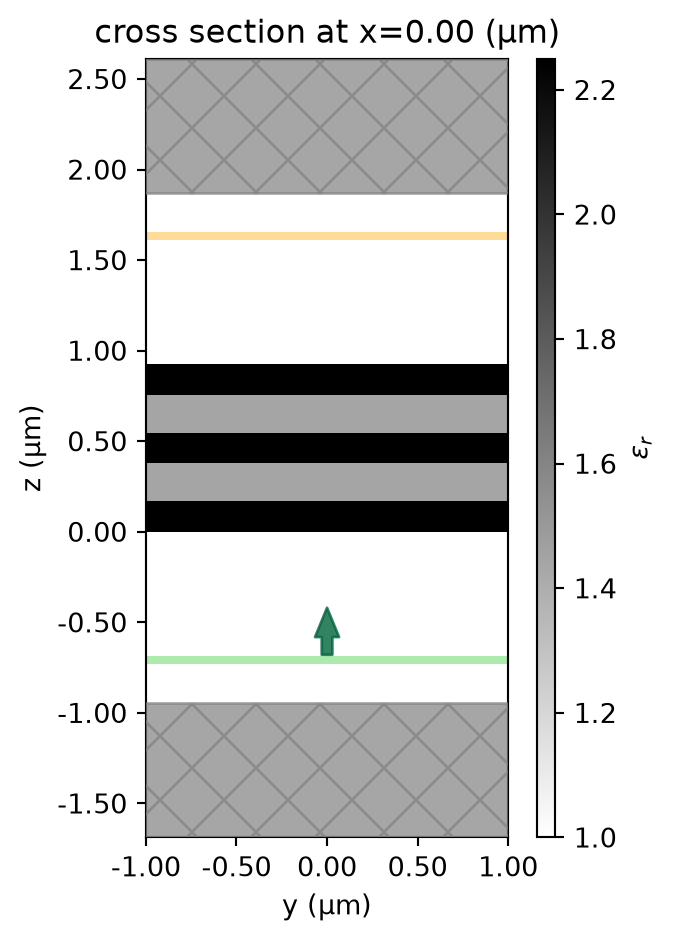
Let’s analyze the transmission of a 1D multilayer slab. Our system will have num layers with refractive index alternating between two values, each with thickness t. We write a function to compute the transmitted flux through this system at frequency freq0 as a function of num and t.

[5]:

lambda0 = 0.63
freq0 = td.C_0 / lambda0

mnt_name = "flux"
buffer = 1.5 * lambda0

refractive_indices = [1.5, 1.2]

We split our simulation process into pre- and post-processing functions so that the Design plugin can handle creating one large Batch, to be run in parallel on the Tidy3D cloud. The pre-processing function returns a tidy3d.Simulation as a function of the input parameters and the post-processing function returns the transmitted flux as a function of the tidy3d.SimulationData associated with the simulation.

[6]:

def pre(num: int, t: float) -> td.Simulation:
    """Pre-processing function, which creates a tidy3d simulation given the function inputs."""
    layers = []
    z = 0
    for i in range(num):
        n = refractive_indices[i % len(refractive_indices)]
        thickness = t * lambda0 / n
        medium = td.Medium(permittivity = n ** 2)
        geometry = td.Box(center=(0, 0, z + thickness / 2), size=(td.inf, td.inf, thickness))
        layers.append(td.Structure(geometry=geometry, medium=medium))
        z += thickness
    Lz = z + 2 * buffer
    sim = td.Simulation(
        size=(0, 0, Lz),
        center=(0, 0, z / 2),
        structures=layers,
        sources=[td.PlaneWave(
            size=(td.inf, td.inf, 0),
            center=(0, 0, -buffer * 0.75),
            source_time=td.GaussianPulse(freq0=freq0, fwidth=freq0/10),
            direction="+",
        )],
        monitors=[td.FluxMonitor(
            size=(td.inf, td.inf, 0),
            center=(0, 0, z + buffer * 0.75),
            freqs=[freq0],
            name=mnt_name,
        )],
        boundary_spec=td.BoundarySpec.pml(x=False, y=False, z=True),
        run_time=100 / freq0,
    )
    return sim

def post(data: td.SimulationData) -> dict:
    """Post-processing function, which processes the tidy3d simulation data to return the function output."""
    flux = np.sum(data['flux'].flux.values)
    return {"flux": flux}

When using MethodMonteCarlo or MethodGrid we can choose to have our post-processing function return a dictionary {"flux": flux} instead of just a float. If a dictionary is returned, the Design plugin will use the keys to label the dataset outputs.

For the optimization tools (MethodBayOpt, MethodGenAlg, MethodParticleSwarm) we must return a float that the optimization can use to evaluate the solution and progress. However, we can return values named as auxiliary data using a notation like [float, dict{"aux1": x}].

Note: if we were to write the full transmission function using pre and post it would look like the function below. However, the Design plugin will handle running the simulation for us, as we’ll see later.

def transmission(num: int, t: float) -> float:
    """Transmission as a function of number of layers and their thicknesses.
         Note: not used, just a demonstration of how the pre and post functions are related.
    """
    sim = pre(num=num, t=t)
    data = web.run(sim, task_name=f"num={num}_t={t}")
    return post(data=data)

Let’s visualize the simulation for some example parameters to make sure it looks ok.

[7]:

sim = pre(num=5, t=0.4)
ax = sim.plot_eps(x=0, hlim=(-1, 1))

Parameters#

We could query these functions directly to perform our own parameter scan, but the advantage of the Design plugin is that it lets us simply define our design problem as a specification and then takes manages the computation for us.

The first step is to define the design “parameters” (or dimensions), which also serve as inputs to our pre function defined earlier.

In this case, we have a parameter num, which is a non-negative integer and a parameter t, which is a positive float.

We can construct a named tdd.Parameter for each of these and define some spans as well. The name fields should correspond to the argument names defined in the pre function.

[8]:

param_num = tdd.ParameterInt(name='num', span=(1, 5))
param_t = tdd.ParameterFloat(name='t', span=(0.1, 0.5), num_points=5)

The float parameter takes an optional num_points option, which tells the design tool how to discretize the continuous dimension only when doing a grid sweep with MethodGrid: for Monte Carlo sweeps, it is not used.

It is also possible to define parameters that are simply sets of quantities that we might want to select using allowed_values, such as:

[9]:

param_str = tdd.ParameterAny(name="some_string", allowed_values=("these", "are", "values"))

but we will ignore this case as it’s not needed here and the internal logic is similar to that for integer parameters.

Note: to do more complex sets of integer parameters (like skipping every ‘n’ integers). We recommend simply using ParameterAny and just passing your integers to allowed_values.

By defining our design parameters like this, we can more concretely define what types and allowed values can be passed to each argument in our function for the parameter sweep.

Method#

Now that we’ve defined our parameters, we also need to define the procedure used to sample the parameter space we’ve defined. As mentioned above, one approach is to independently sample points within the parameter spans, for example using a Monte Carlo method, another is to perform a grid search to uniformly scan between the bounds of each dimension. There are also more complex methods, such as `Bayesian optimization <>`__ and genetic algorithms, which can be seen in these other notebooks.

In the Design plugin, we define the specifications for the parameter sweeps using Method objects.

Here’s one example, which defines a grid search.

[10]:

method = tdd.MethodGrid()

For this example, let’s instead do a Monte Carlo sampling with a set number of points.

[11]:

method = tdd.MethodMonteCarlo(num_points=40)

Design Space#

With the design parameters and our method defined, we can combine everything into a DesignSpace, which is mainly a container that provides some higher level methods for interacting with these objects.

[21]:

design_space = tdd.DesignSpace(parameters=[param_num, param_t], method=method, path_dir="./data", folder_name="Design_Tutorial", task_name="Design_notebook")

We can provide a path_dir to specify the local directory location where files should be stored, and the folder_name which is the location on Tidy3D cloud where the Simulations will be kept.

The task_name argument asigns the root of task name for Tidy3D cloud. This is combined with the index of the Simulation output by the Pre function (often 0) and a counter for the simulations run by the DesignSpace in this format:

{task_name}_{sim_index}_{counter}

If the Pre function outputs Simulation objects as a dictionary then the keys from the dictionary replace the sim_index to be:

{task_name}_{dict_key}_{counter}

Results#

The DesignSpace.run() function returns a Result object, which is basically a dataset containing the function inputs, outputs, source code, and any task ID information corresponding to each data point.

Note that task ID information can only be gathered when using pre and post functions, as in a single function the DesignSpace can’t know which tasks were involved in each data point.

[22]:

results = design_space.run(pre, post)

08:56:24 BST Running 40 Simulations

08:56:25 BST ERROR: The name already exists.                                    

             ERROR: The name already exists.                                    

             ERROR: The name already exists.                                    

             ERROR: The name already exists.                                    

             ERROR: The name already exists.                                    

             ERROR: The name already exists.                                    

             ERROR: The name already exists.                                    

             ERROR: The name already exists.                                    

We can pass verbose=False to the function if we don’t want to see the outputs for large design searches. The “name already exists” error can be ignored here.

Results contains three main related datastructures.

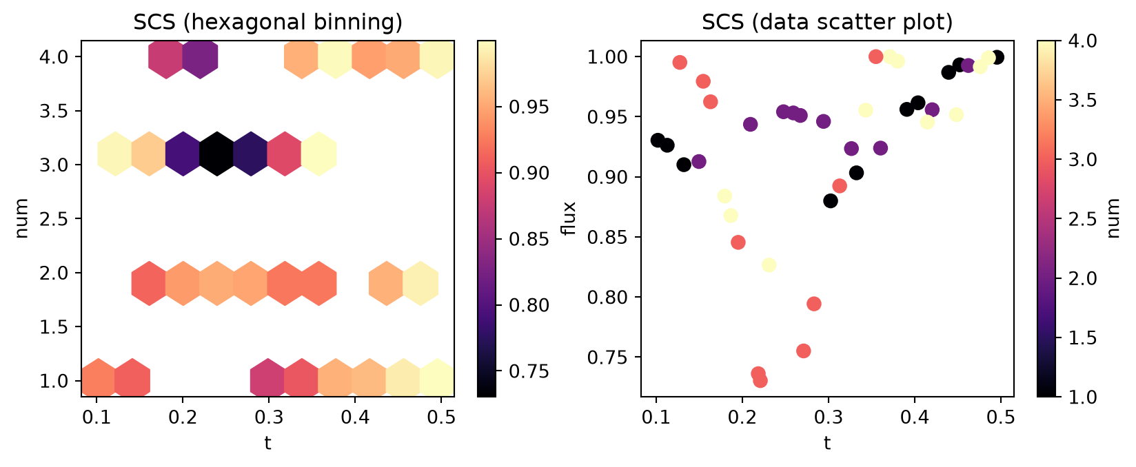
• dims, which correpsond to the kwargs of the pre-processing function, ('num', 't') here.

• coords, which is a tuple containing the values passed in for each of the dims. coords[i] is a tuple of n, and t values for the ith function call.

• values, which is a tuple containing the outputs of the postprocessing functions. In this case values[i] stores the transmission of the ith function call.

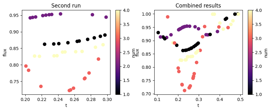
The Results can be converted to a pandas.DataFrame where each row is a separate data point and each column is either an input or output for a function. It also contains various methods for plotting and managing the data.

[14]:

# The first 5 data points
df = results.to_dataframe()
df.head()

[14]:

The pandas documentation provides excellent explanations of the various postprocessing and visualization functions that can be used.

[15]:

f, (ax1, ax2) = plt.subplots(1, 2, figsize=(10, 3.5))

# plot a hexagonal binning of the results
im = df.plot.hexbin(x="t", y="num", gridsize=10, C="flux", cmap="magma", ax=ax1)
ax1.set_title('SCS (hexagonal binning)')

# scatterplot the raw results with flux on the y axis
im = df.plot.scatter(x="t", y="flux", s=50, c="num", cmap="magma", ax=ax2)
ax2.set_title('SCS (data scatter plot)')

plt.show()

These functions just call pandas.DataFrame plotting under the hood, so it is worth referring to the docs page on DataFrame visuazation for more tips on plotting design problem results.

Modifying Results#

After the design problems is run, one might want to modify the results through adding or removing elements or combining different results. Here we will show how to perform some of these advanced features in the Design plugin.

Combining Results#

We can combine the results of two separate design problems assuming they were created with the same functions.

This can be done either with result.combine(other_result) or with a shorthand of result + other_result.

In this example, let’s say we want to explore more the region where the transmission seems to be lowest, for t between 0.2 and 0.3. We create a new parameter with the desired span for t and use it to create an updated copy of the previous design, still using the same method.

[16]:

param_t2 = tdd.ParameterFloat(name='t', span=(0.2, 0.3), num_points=5)
design_space2 = design_space.updated_copy(parameters=[param_num, param_t2])
results2 = design_space2.run(pre, post)

08:34:22 BST Running 40 Simulations

Now we can inspect the new results and the combined data as we did before:

[17]:

results_combined = results + results2

df2 = results2.to_dataframe()
df_combined = results_combined.to_dataframe()

f, (ax1, ax2) = plt.subplots(1, 2, figsize=(10, 3.5))

im = df2.plot.scatter(x="t", y="flux", s=50, c="num", cmap="magma", ax=ax1)
ax1.set_title('Second run')

im = df_combined.plot.scatter(x="t", y="flux", s=50, c="num", cmap="magma", ax=ax2)
ax2.set_title('Combined results')

plt.show()

Adding and removing results#

We can also add and remove individual entries from the Results with the add and delete methods.

Let’s add a new data point to our results and then delete it.

[25]:

# define the function inputs and outputs
fn_args = {"t": 1.2, "num": 5}
value = 1.9

To add a data element, we pass in the fn_args (inputs) and the value (outputs).

[26]:

# add it to the results and view the last 5 entries (data is present)
results = results.add(fn_args=fn_args, value=value)
results.to_dataframe().tail()

[26]:

	num	t	flux
36	3	0.477944	0.995562
37	2	0.383136	0.929275
38	2	0.267950	0.950784
39	3	0.277211	0.773291
40	5	1.200000	1.900000

We can select a specific data point by passing the function inputs as keyword arguments to the Results.sel method.

[27]:

print(results.sel(**fn_args))

1.9

Similarly, we can remove a data point by passing the fn_args (inputs) to the Results.delete method.

[28]:

# remove this data from the results and view the last 5 entries (data is gone)
results = results.delete(fn_args=fn_args)
results.to_dataframe().tail()

[28]:

	num	t	flux
35	1	0.362959	0.930869
36	3	0.477944	0.995562
37	2	0.383136	0.929275
38	2	0.267950	0.950784
39	3	0.277211	0.773291

Leveraging DataFrame functions#

Since we have the ability to convert the Results to and from pandas.DataFrame objects, we are able to perform various manipulations (including the ones above) on the data using pandas. For example, we can create a new DataFrame object that multiplies all of the original flux values by 1/2 and convert this back to a Result if desired.

[29]:

df = results.to_dataframe()
df.head()

[29]:

	num	t	flux
0	4	0.151689	0.946493
1	4	0.427012	0.937147
2	2	0.244466	0.954050
3	2	0.326142	0.923577
4	1	0.484898	0.999998

[30]:

# get a dataframe where everything is squared
df_half_flux = df.copy()
df_half_flux["flux"] = df_half_flux["flux"].map(lambda x: x * 0.5)
df_half_flux.head()

[30]:

	num	t	flux
0	4	0.151689	0.473247
1	4	0.427012	0.468574
2	2	0.244466	0.477025
3	2	0.326142	0.461788
4	1	0.484898	0.499999

We generally recommend you make use of the many features provided by pandas.DataFrame to do further postprocessing and analysis of your sweep results, but to convert a DataFrame back to a Result, one can simply pass it to Results.from_dataframe along with the dimensions of the data (if the DataFrame has been modified).

[25]:

# Load it into a Result, note that we need to pass dims because this is an entirely new DataFrame without metadata
results_squared = tdd.Result.from_dataframe(df_half_flux, dims=("num", "t"))

Accessing Batched Data#

It is possible to load the SimulationData objects from the .hdf5 files that will have been downloaded locally during the DesignSpace.run operation. When using Pre and Post functions the Results object stores the task_names and task_paths to make it easy to identify and load the correct file for further analysis.

[24]:

# See the first three file paths
print(results.task_paths[:3])

# Load the SimulationData back into Python
loaded_sim_data = td.SimulationData.from_file(results.task_paths[0])

['./data/fdve-ba077ef4-b5e0-47ad-bb00-7d991abb089e.hdf5', './data/fdve-e9887d59-1261-433a-a878-f6498c1c3ac4.hdf5', './data/fdve-358eb0f9-f1b9-4362-83a5-16489b5dd7e8.hdf5']

The task_names and task_paths and stored in the same structure as the return from the Pre function to aid with accessing the appropriate SimulationData for a particular output value. For example, if the Pre function returns a list like [Simulation, Simulation, Simulation], then the task_paths will be stored as a list of corresponding paths: [path, path, path].

Working with Optimizers#

Using a grid search or Monte Carlo are good ways to sample a large design space. However, the Design plugin can go further and enable efficient optimization of a design problem using a range of different optimization techniques. Method objects such as Bayesian optimization, genetic algorithms, and partical swarm optimization can all be used in the same way as the above examples. These methods use a float value output by the post function to evaluate the effectiveness of a solution, and then propose new solutions that should prove better. More detailed examples can be found in the notebooks associated with each technique.

1. Bayesian Optimization of Y-Junction

2. Particle Swarm Optimizer PBS

3. Particle Swarm Optimizer Bullseye Cavity

4. Genetic Algorithm Reflector

There are a few additional points to consider when using optimizers:

• Optimizers are more complicated to use than samplers and have many different options to consider in the Method object. It is worth reading the Tidy3D docs and relevant package documentation for each optimizer before use.

• Optimizers require the output of fn_post to be either a float or [float, list/tuple/dict]. The additional information in the container will be handled as auxiliary data and stored in the Results. It can be added to the pd.DataFrame with results.to_dataframe(include_aux=True).

• Optimizers work best when the design problem is split into pre and post functions as the DesignSpace can create efficient batches of Simulation objects, instead of running the entire optimization process sequentially, which can take a long time.