Fitting dispersive material models#

Here we show how to fit optical measurement data and use the results to create dispersion material models for Tidy3D.

Tidy3D’s dispersion fitting tool peforms an optimization to find a medium defined as a dispersive PoleResidue model that minimizes the RMS error between the model results and the data. This can then be directly used as a material in simulations.

If you are new to the finite-difference time-domain (FDTD) method, we highly recommend going through our FDTD101 tutorials. For simulation examples, please visit our examples page. If you are new to the finite-difference time-domain (FDTD) method, we highly recommend going through our FDTD101 tutorials. FDTD simulations can diverge due to various reasons. If you run into any simulation divergence issues, please follow the steps outlined in our troubleshooting guide to resolve it.

We recommend using the FastDispersionFitter, with advanced options configurable using the AdvancedFastFitterParam.

[1]:

# first import packages
import matplotlib.pylab as plt
import numpy as np

import tidy3d as td

Load Data#

The fitting tool accepts three ways of loading data:

Numpy arrays directly by specifying wvl_um, n_data, and optionally k_data;
Data file with the from_file utility function.

Our data file has columns for wavelength (um), real part of refractive index (n), and imaginary part of refractive index (k). k data is optional.

Note: from_file uses np.loadtxt under the hood, so additional keyword arguments for parsing the file follow the same format as np.loadtxt.
URL linked to a csv/txt file that contains wavelength (micron), n, and optionally k data with the from_url utility function. URL can come from refractiveindex.info.

Below the 2nd way is taken as an example:

[2]:

from tidy3d.plugins.dispersion import FastDispersionFitter, AdvancedFastFitterParam

fname = "misc/nk_data.csv"

# note that additional keyword arguments to load_nk_file get passed to np.loadtxt
fitter = FastDispersionFitter.from_file(fname, skiprows=1, delimiter=",")

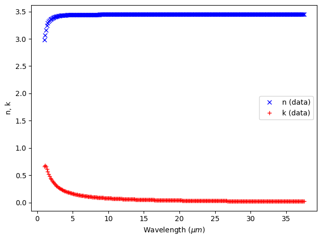
# lets plot the data
fitter.plot()
plt.show()

Fitting the data#

The fitting tool fit a dispersion model to the data by minimizing the root mean squared (RMS) error between the model n,k prediciton and the data at the given wavelengths.

There are various fitting parameters that can be set, but the most important is the number of “poles” in the model.

For each pole, there are 4 degrees of freedom in the model. Adding more poles can produce a closer fit, but each additional pole added will make the fit harder to obtain and will slow down the FDTD. Therefore, it is best to try the fit with few numbers of poles and increase until the results look good.

Here, we will first try fitting the data with 1 pole and specify the RMS value that we are happy with (tolerance_rms).

We specify weights for the real and imaginary part of the permittivity using AdvancedFastFitterParam, although the default weights which are calculated based on the typical values would also work fine here. Also note that, by default, eps_inf is optimized, although alternatively a fixed value for eps_inf can be specified as an argument to fitter.fit.

[3]:

advanced_param = AdvancedFastFitterParam(weights=(1,1))
medium, rms_error = fitter.fit(max_num_poles=1, advanced_param=advanced_param, tolerance_rms=2e-2)
fitter.plot(medium)
plt.show()

Best weighted RMS error so far: 0.0295 ━━━━━━━━━━━━━━━━━━━━━━━━━━━━ 100% 0:00:00

10:48:22 EDT WARNING: Unable to fit with weighted RMS error under               
             'tolerance_rms' of 0.02

The RMS error was above our tolerance and there is room for improvement at short wavelengths, so we might want to try more fits.

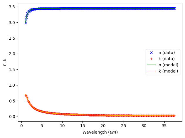
Let’s now try a fit with up to 3 poles.

[4]:

medium, rms_error = fitter.fit(max_num_poles=3, advanced_param=advanced_param, tolerance_rms=2e-2)
fitter.plot(medium)
plt.show()

Best weighted RMS error: 0.0114 ━━━━━━━━━━━━━━━━━━━━━━━━━━━━━━━━━━━ 100% 0:00:00

This fit looks great and should be sufficient for our simulation.

Alternatively, if the simulation is narrowband, you might want to truncate your data to not include wavelengths far outside your measurement wavelength to simplify the dispersive model. This is through modifying the attribute wvl_range where you can set the lower wavelength bound wvl_range[0] and the higher wavelength bound wvl_range[1]. This operation is non-destructive, so you can always unset them by setting the value to None.

E.g. if we are only interested in the wavelength 3-20 um, we can still use the single-pole model:

[5]:

fitter = fitter.copy(update={"wvl_range": (3, 20)})
medium, rms_error = fitter.fit(max_num_poles=1, tolerance_rms=2e-2)

Best weighted RMS error: 0.000114 ━━━━━━━━━━━━━━━━━━━━━━━━━━━━━━━━━ 100% 0:00:00

[6]:

fitter.plot(medium)
plt.show()

Using Fit Results#

With the fit performed, we want to use the Medium in our simulation.

Method 1: direct export as Medium#

The fit returns a medium, which can be used directly in simulation

[7]:

b = td.Structure(geometry=td.Box(size=(1, 1, 1)), medium=medium)

Method 2: print medium definition string#

In many cases, one may want to perform the fit once and then hardcode the result in their tidy3d script.

For a quick and easy way to do this, just print() the medium and the output can be copied and pasted into your main svript

[8]:

print(medium)

td.PoleResidue(
        eps_inf=3.3946193815575816,
        poles=(((-1667817350156664.2-206849778478069.44j), (1.004708275108366e+16-2.3076845274369316e+16j)),),
        frequency_range=None)

[9]:

# medium = td.PoleResidue(
#   eps_inf=3.394619381557077,
#   poles=(((-1667817350156741.8-206849778477574.28j), (1.004708275108508e+16-2.307684527443524e+16j)),),
#   frequency_range=None)

Method 3: save and load file containing poles#

Finally, one can save export the Medium directly as .json file. Here is an example.

[10]:

# save poles to pole_data.txt
fname = "misc/my_medium.json"
medium.to_file(fname)

# load the file in your script
medium = td.PoleResidue.from_file(fname)

Advanced Parameters and Tips for FastDispersionFitter#

There are a number of advanced parameters for the FastDispersionFitter which can be useful if the default settings do not work to find a fit. The advanced parameters are configured by passing in an AdvancedFastFitterParam object. When trying to improve a fit, the first thing to try is changing the arguments max_num_poles and eps_inf to the fit function. Importantly, although eps_inf = None performs optimization for the value of eps_inf as well, this optimization is nontrivial and so it can sometimes be better to provide a fixed value of eps_inf. Besides these arguments, the following advanced parameters may be helpful:

loss_bounds = (lower, upper) are bounds on Im[eps] over all frequencies (not just the fitting range). The default (0, np.inf) corresponds to a passive medium requirement, which leads to stable simulations. The upper bound can be used to ensure a good fit for a lossless medium. Setting a small negative lower bound can sometimes be informative; if a lower bound of 0 results in a poor fit but a small negative lower bound results in a good fit, then the poor fit was due to difficulty satisfying the passivity requirement. A negative lower bound, and thus a violation of the passivity requirement, may result in unstable simulations. However, a small violation of the passivity requirement may on occasion be acceptable, if there is loss elsewhere in the simulation to offset the resulting gain.
weights = (real, imag) are weights for Re[eps] and Im[eps] used in the fitting objective function (and when reporting rms error). These can be used if it is necessary to more accurately fit either the real or imaginary part.
relaxed, smooth, and logspacing can usually be left at their default values of None, which makes the fitter try both True and False values and take the better fit. Sometimes, however, it may be clear that specific values are better for a certain medium. relaxed controls whether the relaxed version of the fitting algorithm is used. For example, relaxed = True could prevent overfitting and also allow for pole relocation further outside the fitting window. The smooth and logspacing parameters control the initial pole placement. smooth = True may be appropriate for fitting metals. logspacing = True may be better when the poles are spread over a large frequency range. Again, the default option is usually fine here unless a particular type of model is required, since the default option tries both True and False.
num_iters controls the tradeoff between speed and quality of fit, although a higher num_iters doesn’t necessarily result in a better fit. Usually, after a certain number of iterations, the algorithm has converged to a certain fit, and increasing num_iters further won’t significantly help. However, it may be good to try increasing it to 100 or so to make sure that the algorithm has converged.

Information on additional advanced parameters may be found in the documentation here.

Here are a couple more general tips on dispersion fitting:

If you are unable to find a good fit to your data, it might be worth considering whether you care about certain features in the data. For example as shown above, if the simulation is narrowband, you might want to truncate your data to not include wavelengths far outside your measurement wavelength to simplify the dispersive model.
It is common to find divergence in FDTD simulations due to dispersive materials. The FastDispersionFitter by default should enforce a passivity requirement and produce stable material fits. If there is still a divergence, besides trying “absorber” PML types and reducing runtime, a good solution can be to try other fits; for example, using a smaller number of poles, or setting loss_bounds = (min_loss, np.inf) for some small positive number min_loss (the latter can only work if the data satisfies this minimum loss constraint).

Fitting dispersive material models

Contents