
Analytic Directional Coupler Model

A directional coupler (DC) is one of the fundamental building blocks in integrated photonics. Two waveguides brought into close proximity exchange optical power through evantiescent coupling. PhotonForge provides the AnalyticDirectionalCouplerModel to capture this behaviour with a small set of physically meaningful parameters, making it ideal for fast circuit-level design exploration.
This notebook focuses on three key lengths that govern the analytic model:
Symbol |
Name |
Meaning |
|---|---|---|
\(l_i\) |
Interaction length |
Physical length over which the two waveguides are close enough for coupling. This is a geometric parameter determined by your layout. |
\(l_c\) |
Coupling length (beat length) |
Length required for complete (100 %) power transfer from one waveguide to the other. It depends on waveguide geometry, gap, and wavelength. |
\(l_p\) |
Propagation length |
Effective optical path length used for phase accumulation. Defaults to \(l_i\) when not specified; set it differently when S-bends add extra path. |
After exploring these concepts we will create a real directional coupler, simulate it with FDTD, and show that the AnalyticDirectionalCouplerModel can reproduce both the magnitude and phase of the FDTD S parameters.
Setup
[1]:
import matplotlib.pyplot as plt
import numpy as np
import tidy3d as td
import photonforge as pf
[2]:
tech = pf.basic_technology(strip_width=0.4)  # narrower strip for stronger evanescent coupling
pf.config.default_technology = tech

wavelengths = np.linspace(1.5, 1.6, 101)
freqs = pf.C_0 / wavelengths
Understanding the Three Lengths
Coupling ratio
The power coupling ratio from the bar (through) port to the cross port is:
When \(l_i = l_c\) the argument of the sine equals \(\pi/2\), so \(c_r = 1\) (complete crossover). When \(l_i = l_c / 2\) we get \(c_r = 0.5\) (3-dB splitter).
Interaction length \(l_i\)
The interaction length is the physical length over which the waveguides are close enough for evanescent coupling. Increasing \(l_i\) increases the coupling ratio sinusoidally until full crossover at \(l_i = l_c\). Beyond that, power couples back to the bar port.
Coupling length \(l_c\) (beat length)
The coupling length (also called the beat length) is the length at which complete power transfer occurs. It is not a layout parameter — it is determined by the gap, waveguide geometry, and wavelength. A smaller gap produces a shorter \(l_c\).
Propagation length \(l_p\)
The propagation length controls only the accumulated phase:
By default \(l_p = l_i\). However, when S-bends or tapers add extra optical path before and after the straight coupling section, \(l_p\) should be set to the total optical path through the coupler.
Exploring the Analytic Model
We use AnalyticDirectionalCouplerModel with black_box_component to quickly create test components without defining a physical layout. This lets us sweep parameters and build intuition before committing to a geometry.
We start with a 50/50 coupler design: \(l_i = l_c / 2\).
[3]:
coupling_length = 20.0  # µm — beat length for our waveguide/gap combination

model_50 = pf.AnalyticDirectionalCouplerModel(
    interaction_length=coupling_length / 2,
    coupling_length=coupling_length,
    n_eff=2.4,
    n_group=4.2,
)

bb_50 = model_50.black_box_component(port_spec="Strip")
bb_50
[3]:

From here, it’s easy to see the s matrix of this component:
[4]:
s_50 = bb_50.s_matrix(freqs)
pf.plot_s_matrix(s_50)
plt.suptitle("50/50 coupler ($l_i = l_c/2$) — Magnitude", y=1.02)
plt.show()
Progress: 100%
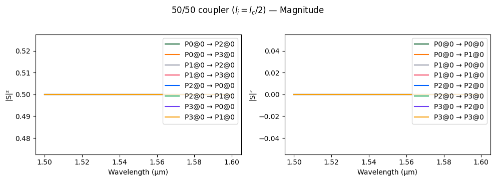
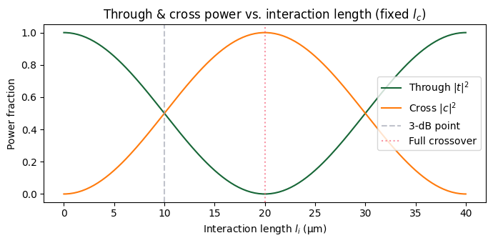
The through and cross ports carry equal power — this is the ideal 3-dB splitter. Now let’s see what happens when we sweep the interaction length from 0 to \(2 l_c\).
[5]:
f0 = pf.C_0 / 1.55
interaction_lengths = np.linspace(0, 2 * coupling_length, 201)
cr_sweep = np.sin(np.pi * interaction_lengths / (2 * coupling_length)) ** 2

fig, ax = plt.subplots(figsize=(7, 3.5))
ax.plot(interaction_lengths, 1 - cr_sweep, label="Through $|t|^2$")
ax.plot(interaction_lengths, cr_sweep, label="Cross $|c|^2$")
ax.axvline(coupling_length / 2, color="C2", linestyle="--", alpha=0.6, label="3-dB point")
ax.axvline(coupling_length, color="C3", linestyle=":", alpha=0.6, label="Full crossover")
ax.set_xlabel("Interaction length $l_i$ (µm)")
ax.set_ylabel("Power fraction")
ax.set_title("Through & cross power vs. interaction length (fixed $l_c$)")
ax.legend(loc="center right")
fig.tight_layout()
plt.show()
Effect of propagation length on phase
The propagation length \(l_p\) does not affect the power splitting — it only changes the accumulated phase \(\phi\) on both the through and cross coefficients. Below we compare the phase of the through port for two models that differ only in \(l_p\): one is \(l_c/2\), the other is \(l_c/2 + 5\).
[6]:
li = coupling_length / 2

model_lp_equal = pf.AnalyticDirectionalCouplerModel(
    interaction_length=li,
    coupling_length=coupling_length,
    propagation_length=li,
    n_eff=2.4,
    n_group=4.2,
)

model_lp_longer = pf.AnalyticDirectionalCouplerModel(
    interaction_length=li,
    coupling_length=coupling_length,
    propagation_length=li + 5,
    n_eff=2.4,
    n_group=4.2,
)

bb_eq = model_lp_equal.black_box_component(port_spec="Strip")
bb_lg = model_lp_longer.black_box_component(port_spec="Strip")

s_eq = bb_eq.s_matrix(freqs)
s_lg = bb_lg.s_matrix(freqs)

port_names = sorted(s_eq.ports)
through_key = (f"{port_names[0]}@0", f"{port_names[2]}@0")

fig, axes = plt.subplots(1, 2, figsize=(12, 4))

ax = axes[0]
ax.plot(wavelengths, np.abs(s_eq[through_key]) ** 2, label="$l_p = l_i$")
ax.plot(wavelengths, np.abs(s_lg[through_key]) ** 2, "--", label="$l_p = l_i + 5$")
ax.set_xlabel("Wavelength (µm)")
ax.set_ylabel("$|t|^2$")
ax.set_title("Through power (identical)")
ax.legend()

ax = axes[1]
ax.plot(wavelengths, np.unwrap(np.angle(s_eq[through_key])), label="$l_p = l_i$")
ax.plot(wavelengths, np.unwrap(np.angle(s_lg[through_key])), "--", label="$l_p = l_i + 5$")
ax.set_xlabel("Wavelength (µm)")
ax.set_ylabel("Phase (rad)")
ax.set_title("Through phase (different)")
ax.legend()

fig.tight_layout()
plt.show()
Progress: 100%
Progress: 100%
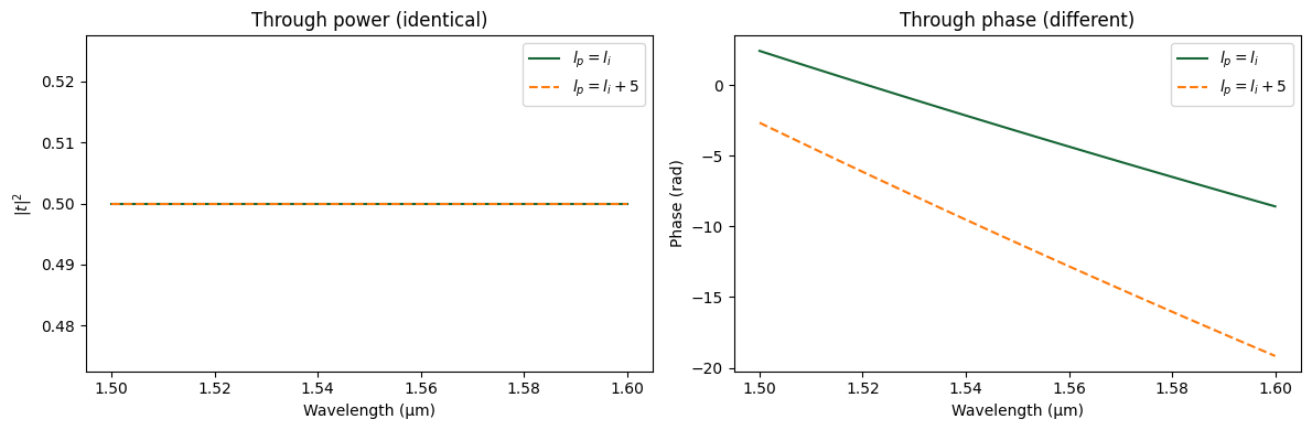
The left panel confirms that the power splitting is unchanged — \(l_p\) has no effect on magnitude. The right panel shows that the additional 5 µm of propagation length introduces extra phase accumulation. This distinction is critical: in a layout with S-bends the waveguides travel a longer optical path than the straight coupling section alone, and the propagation_length parameter lets us capture that extra phase.
Creating a Real Directional Coupler
We now create an actual directional coupler layout using pf.parametric.dual_ring_coupler and simulate it with Tidy3D’s FDTD solver. We use a narrower strip (strip_width=0.4 µm) so that coupling is stronger and a compact device can be designed.
[7]:
port_spec = tech.ports["Strip"]
core_width = port_spec.path_profiles_list()[0][0]
gap = 0.2
coupling_distance = core_width + gap

dc = pf.parametric.dual_ring_coupler(
    port_spec="Strip",
    coupling_distance=coupling_distance,
    radius=5,
    coupling_length=4,
)
dc
[7]:

FDTD Simulation
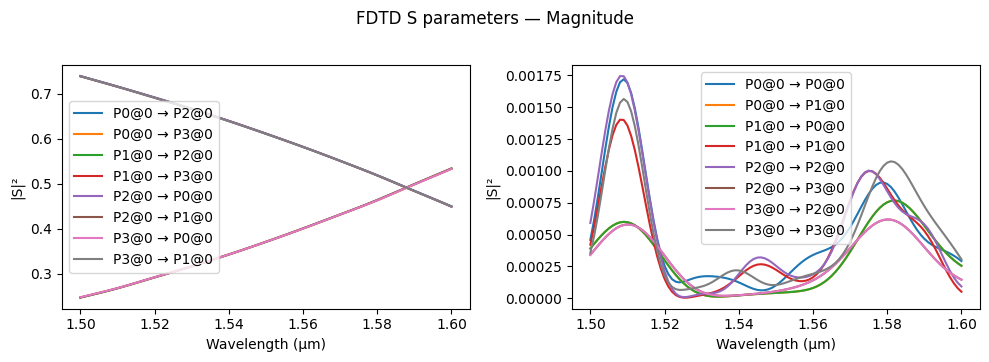
We compute the S matrix of the directional coupler using Tidy3D’s FDTD solver.
[8]:
s_fdtd = dc.s_matrix(freqs)
pf.plot_s_matrix(s_fdtd)
plt.suptitle("FDTD S parameters — Magnitude", y=1.02)
plt.show()
Uploading task 'P0@0…'
Uploading task 'X0@0…'
Uploading task 'P1@0…'
Uploading task 'X1@0…'
Uploading task 'P2@0…'
Uploading task 'X2@0…'
Uploading task 'P3@0…'
Uploading task 'X3@0…'
Uploading task 'P0@0…'
Uploading task 'P1@0…'
Uploading task 'P2@0…'
Uploading task 'P3@0…'
Starting task 'P0@0': https://tidy3d.simulation.cloud/workbench?taskId=fdve-db31cd39-bec7-4416-a802-5c4854f38840
Starting task 'X0@0': https://tidy3d.simulation.cloud/workbench?taskId=fdve-08839622-fcdf-4f80-a8dc-3e0da1965a67
Downloading data from 'P0@0'…
Downloading data from 'X0@0'…
Starting task 'P1@0': https://tidy3d.simulation.cloud/workbench?taskId=fdve-25fd667a-224c-4f45-a3ee-5369e4d622bf
Starting task 'X1@0': https://tidy3d.simulation.cloud/workbench?taskId=fdve-86de585a-055d-413d-9586-0acb743418ee
12:36:01 -03 WARNING: Warning messages were found in the solver log. For more
             information, check 'SimulationData.log' or use
             'web.download_log(task_id)'.
Downloading data from 'P1@0'…
Downloading data from 'X1@0'…
Starting task 'P2@0': https://tidy3d.simulation.cloud/workbench?taskId=fdve-1b8849ec-fb53-46bc-8e1c-9c946906eaec
Starting task 'X2@0': https://tidy3d.simulation.cloud/workbench?taskId=fdve-58e90a65-ea7d-4fcb-a974-a3bad108a06a
Starting task 'X3@0': https://tidy3d.simulation.cloud/workbench?taskId=fdve-8b5c2a1f-8f21-42d1-b633-926292663e68
Downloading data from 'P2@0'…
Downloading data from 'X2@0'…
Starting task 'P0@0': https://tidy3d.simulation.cloud/workbench?taskId=fdve-85264eb8-c149-4efc-a2c4-5f426cc72819
Progress: 14% |
12:36:08 -03 WARNING: Warning messages were found in the solver log. For more
             information, check 'SimulationData.log' or use
             'web.download_log(task_id)'.
Downloading data from 'X3@0'…
Starting task 'P2@0': https://tidy3d.simulation.cloud/workbench?taskId=fdve-bd756d6f-0548-48b8-b999-ab0ba6f75faa
Starting task 'P3@0': https://tidy3d.simulation.cloud/workbench?taskId=fdve-d09b22b2-730e-47aa-8d7c-875eaf3d43c0
Downloading data from 'P0@0'…
Starting task 'P1@0': https://tidy3d.simulation.cloud/workbench?taskId=fdve-aa407e83-769e-49e9-b06a-0ef6310d8bbd
Downloading data from 'P2@0'…
Downloading data from 'P3@0'…
Starting task 'P3@0': https://tidy3d.simulation.cloud/workbench?taskId=fdve-91ce60ed-77ab-4da5-a213-90b34e351e5f
Downloading data from 'P1@0'…
Downloading data from 'P3@0'…
Progress: 100%
[9]:
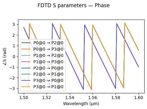
pf.plot_s_matrix(s_fdtd, y="phase")
plt.suptitle("FDTD S parameters — Phase", y=1.02)
plt.show()
Fitting the Analytic Model to FDTD Results
We now extract the analytic model parameters from the FDTD S matrix. The procedure is:
Compute the insertion loss \(L_\text{dB} = -20 \log_{10}(\sqrt{|t|^2 + |c|^2})\) and the coupling ratio \(c_r(\lambda) = |c|^2 / (|t|^2 + |c|^2)\) (normalising out insertion loss).
Estimate \(l_c\) from \(c_r\) at the centre wavelength: \(l_c = \pi l_i \,/\, [2 \arcsin(\sqrt{c_r})]\).
Obtain \(n_\text{eff}\) and \(n_\text{group}\) from running Tidy3D’s modesolver.
Determine the cross-phase shift \(\Delta\phi\) from the phase difference between the cross and through ports.
Step 1 — Compute coupling ratio and insertion loss
[10]:
t_fdtd = s_fdtd[('P0@0', 'P2@0')]
c_fdtd = s_fdtd[('P0@0', 'P3@0')]

T2 = np.abs(t_fdtd) ** 2
C2 = np.abs(c_fdtd) ** 2
total_power = T2 + C2

insertion_loss_dB = -10 * np.log10(total_power)
cr_fdtd = C2 / total_power
Step 2 — Estimate \(l_c\) from \(c_r\) at the center wavelength
[11]:
i_center = len(wavelengths) // 2
cr_center = cr_fdtd[i_center]
il_center = insertion_loss_dB[i_center]

li_est = dc.parametric_kwargs["coupling_length"]

lc_est = np.pi * li_est / (2 * np.arcsin(np.sqrt(cr_fdtd)))

print(f"Estimated interaction length l_i: {li_est:.2f} µm")
print(f"Coupling length l_c at centre:    {lc_est[i_center]:.2f} µm")
print(f"Coupling length l_c range:        [{lc_est.min():.2f}, {lc_est.max():.2f}] µm")
Estimated interaction length l_i: 4.00 µm
Coupling length l_c at centre:    9.50 µm
Coupling length l_c range:        [7.59, 11.98] µm
Step 3 — Obtain \(n_\text{eff}\), \(n_\text{group}\), and propagation length
We obtain the effective and group indices directly from the waveguide mode solver, which gives physically meaningful values. The propagation length \(l_p\) is computed from the actual geometry: two S-bends (totalling a half-circle arc of \(\pi R\)) plus the straight coupling section.
[12]:
f0 = freqs[i_center]

mode_data = pf.port_modes("Strip", [f0], group_index=True)
n_eff_est = float(mode_data.data.n_eff.isel(mode_index=0).values[0])
n_group_est = float(mode_data.data.n_group.isel(mode_index=0).values[0])

radius = 5  # from dual_ring_coupler call
coupling_len = dc.parametric_kwargs["coupling_length"]
lp_est = radius * np.pi + coupling_len

print(f"n_eff (mode solver):   {n_eff_est:.4f}")
print(f"n_group (mode solver): {n_group_est:.4f}")
print(f"Propagation length l_p: {lp_est:.2f} µm  (π·R + coupling_length)")
Uploading task 'Mode-ModeSolver…'Progress: 0% -
Starting task 'Mode-ModeSolver': https://tidy3d.simulation.cloud/workbench?taskId=mo-75378205-f806-4496-80bf-327437af540e
Downloading data from 'Mode-ModeSolver'…
Progress: 100%
n_eff (mode solver):   2.2224
n_group (mode solver): 4.3677
Propagation length l_p: 19.71 µm  (π·R + coupling_length)
Step 4 — Estimate cross-port phase shift \(\Delta\phi\)
The cross-phase shift is the phase offset between the cross and through coefficients, after factoring out the common propagation phase.
[13]:
phi_through = np.unwrap(np.angle(t_fdtd))
phi_cross = np.unwrap(np.angle(c_fdtd))
delta_phi = phi_cross[i_center] - phi_through[i_center]
delta_phi_deg = np.rad2deg(delta_phi)

print(f"Estimated cross-phase shift Δφ: {delta_phi_deg:.2f}°")
Estimated cross-phase shift Δφ: 270.43°
Build the analytic model and compare
We construct an AnalyticDirectionalCouplerModel with the extracted parameters and overlay its S matrix on the FDTD results. Note that we must define a reference_frequency in order to do this; n_eff and n_group must be evaluated at this frequency for correct dispersion modeling.
We also add an empirically tested phase offset in order to get the phases to match.
[14]:
phi0 = np.pi * 1.1 # empirical phase offset

analytic_model = pf.AnalyticDirectionalCouplerModel(
    interaction_length=li_est,
    coupling_length=lc_est.reshape(1, -1),
    propagation_length=lp_est,
    cross_phase=delta_phi_deg,
    insertion_loss=il_center,
    n_eff=n_eff_est,
    n_group=n_group_est,
    reference_frequency=f0,
    ports=sorted(s_fdtd.ports),
)

bb_fit = analytic_model.black_box_component(port_spec="Strip")
s_analytic = bb_fit.s_matrix(freqs)

print("Analytic model created successfully.")
Analytic model created successfully.Starting…
Progress: 100%
[15]:
port_names_a = sorted(s_analytic.ports)
through_key_a = (f"{port_names_a[0]}@0", f"{port_names_a[2]}@0")
cross_key_a = (f"{port_names_a[0]}@0", f"{port_names_a[3]}@0")
t_analytic = s_analytic[through_key_a]
c_analytic = s_analytic[cross_key_a]
fig, axes = plt.subplots(2, 2, figsize=(12, 8))
ax = axes[0, 0]
ax.plot(wavelengths, np.abs(t_fdtd) ** 2, label="FDTD")
ax.plot(wavelengths, np.abs(t_analytic) ** 2, "--", label="Analytic")
ax.set_ylabel("$|t|^2$")
ax.set_title("Through — Power")
ax.legend()
ax = axes[0, 1]
ax.plot(wavelengths, np.abs(c_fdtd) ** 2, label="FDTD")
ax.plot(wavelengths, np.abs(c_analytic) ** 2, "--", label="Analytic")
ax.set_ylabel("$|c|^2$")
ax.set_title("Cross — Power")
ax.legend()
ax = axes[1, 0]
ax.plot(wavelengths, np.unwrap(np.angle(t_fdtd)), label="FDTD")
ax.plot(wavelengths, np.unwrap(np.angle(t_analytic*np.exp(1j*phi0))), "--", label="Analytic")
ax.set_xlabel("Wavelength (µm)")
ax.set_ylabel("Phase (rad)")
ax.set_title("Through — Phase")
ax.legend()
ax = axes[1, 1]
ax.plot(wavelengths, np.unwrap(np.angle(c_fdtd)), label="FDTD")
ax.plot(wavelengths, np.unwrap(np.angle(c_analytic*np.exp(1j*phi0))), "--", label="Analytic")
ax.set_xlabel("Wavelength (µm)")
ax.set_ylabel("Phase (rad)")
ax.set_title("Cross — Phase")
ax.legend()
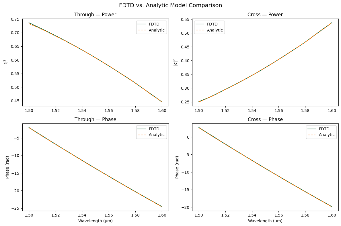
fig.suptitle("FDTD vs. Analytic Model Comparison", fontsize=14)
fig.tight_layout()
plt.show()
Replacing the FDTD model
Once we are satisfied with the fit, we can assign the analytic model to the component. This makes circuit-level simulations (e.g. MZI, ring resonators) orders of magnitude faster when exploring new interaction lengths, since no additional FDTD runs are needed. (For previously simulated geometries, FDTD results are cached and already fast to retrieve.)
[16]:
dc.add_model(analytic_model, "AnalyticDC", set_active=True)

s_fast = dc.s_matrix(freqs)
print("Active model:", dc.active_model)
pf.plot_s_matrix(s_fast)
plt.suptitle("Directional coupler with analytic model", y=1.02)
plt.show()
 AnalyticDirectionalCouplerModel
Progress: 100%
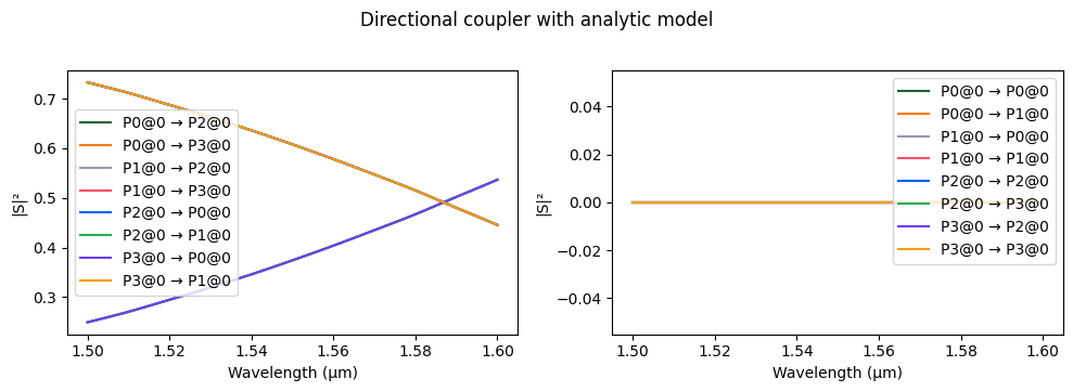
Thus the AnalyticDirectionalCouplerModel can reproduce FDTD results with high fidelity in both magnitude and phase. When exploring new interaction lengths or coupling parameters, it is orders of magnitude faster than running new FDTD simulations, making it the ideal choice for design exploration and circuit simulation.