Quantum Chip Simulation

This notebook implements a generalized, physics-accurate simulation of a programmable quantum photonic processor. It models a cascaded mesh of Mach-Zehnder Interferometers (MZIs) designed to act as a quantum matched filter. Given an arbitrary \(N\)-dimensional quantum superposition (the target_state), the algorithm calculates the exact phase-shifter voltages required to reverse-propagate that state, constructively interfering 100% of the photon’s amplitude into a single target
detector.
Bridging the gap between theoretical quantum algorithms and physical photonics is notoriously difficult. Theoretical math assumes perfect 50:50 beam splitters and identical waveguides. The physical world contains splitting imbalances, asymmetric path lengths, and thermal crosstalk.
This script is built as a “Digital Twin” of the physical hardware, simulating the exact experimental control procedures used in modern quantum photonics labs to overcome these hardware realities.
Core Architecture & Features
Algorithmic Reverse-Propagation: Implements the Vector Element Elimination algorithm. It recursively traverses the \(\log_2(N)\) layers of the optical tree, calculating the precise amplitude ratios (\(\theta\)) and phase alignments (\(\phi\)) required at every MZI junction to “un-split” the target state.
Empirical “Digital Twin” Physics: Rather than using ideal textbook equations, the algorithm derives its complex transfer matrices dynamically from actual FDTD-simulated S-matrix data of the projector circuit. This allows the algorithm to inherently “know” and compensate for real-world manufacturing imperfections (like an MMI 50:47 splitting ratio).
Automated Hardware Calibration: Replicates the laboratory routine of “fringe scanning.” Before running any quantum logic, the script sweeps the physical chip to measure and record the intrinsic, arbitrary phase delays of the zig-zagging silicon waveguides, creating a baseline to subtract from the theoretical quantum phases.
Thermal Noise Injection: Simulates realistic experimental degradation by injecting customizable Gaussian noise (\(\sigma\)) into the heater temperatures. This models both the digital-to-analog converter (DAC) inaccuracies and the thermal crosstalk between adjacent phase shifters.
Comprehensive Validation: Automatically evaluates the simulated processor’s operational fidelity against two distinct quantum bases:
Z-Basis (Computational): Tests the classical routing and amplitude control.
F-Basis (Fourier): A rigorous stress test of the chip’s phase stability, requiring multiple paths to perfectly interfere simultaneously.
References:
Wang, Jianwei, et al. “Multidimensional quantum entanglement with large-scale integrated optics.” Science 2018 360 (6386), 285-291. doi: 10.1126/science.aar7053
[1]:
%%capture
# Download the following notebooks before running:
# https://docs.flexcompute.com/projects/photonforge/en/latest/examples/Quantum_Chip_Layout.html
# https://docs.flexcompute.com/projects/photonforge/en/latest/examples/Quantum_Chip_Components.html
%run Quantum_Chip_Layout.ipynb
Progress: 100%
Progress: 100%
Progress: 100%
Progress: 100%
Step 1: Hardware Setup and Physical Mapping
Before executing the quantum phase-elimination algorithm, we must map the abstract mathematical dimensions to the physical layout of our simulated chip.
This initialization cell performs three critical setup tasks:
Dynamic Targeting: It locks onto the exact frequency index of the idler photon (bypassing the input AMZI wavelength splitters) and dynamically assigns the target detector port (
P{n_src}) based on the chosen projection dimension \(d\).Topology Extraction (
get_alice_mzi_indices): Because the physical layout interleaves Alice’s and Bob’s interferometers column-by-column, this function mathematically traverses the binary tree to extract the specific hardware indices belonging only to Alice’s state projector.Realistic Hardware Driver (
phase_to_temp): This function bridges the gap between quantum theory and experimental reality. It maps ideal mathematical phase shifts (radians) to physical heater temperatures (Kelvin) based on our CROSS/BAR calibration. Crucially, it injects Gaussian thermal noise to accurately simulate real-world experimental limits, such as digital-to-analog converter (DAC) inaccuracies and thermal crosstalk between adjacent silicon phase shifters.
[2]:
# Temperature noise level in Kelvin
noise_level = 1.0

mzi_n = mzi.name
tps_n = tps.name
freq_idx = np.argmin(np.abs(wavelengths - idler_wavelength))
target_port = f"P{n_src}@0"

def get_alice_mzi_indices(n_src):
    indices = []
    current_start = 0
    mzis_in_layer = n_src
    while mzis_in_layer >= 2:
        alice_mzis_in_this_layer = mzis_in_layer // 2
        for i in range(alice_mzis_in_this_layer):
            indices.append(current_start + i)
        current_start += mzis_in_layer
        mzis_in_layer //= 2
    return indices

alice_tps_indices = sorted_indices[:n_src]
alice_mzi_indices = get_alice_mzi_indices(n_src)

def phase_to_temp(phase_rad, temp_noise_std=0.0):
    """Converts a phase shift to temperature, injecting Gaussian thermal noise."""
    phase_rad = phase_rad % (2 * np.pi)
    ideal_temp = T_CROSS + (phase_rad / np.pi) * (T_BAR - T_CROSS)

    if temp_noise_std > 0:
        return np.random.normal(loc=ideal_temp, scale=temp_noise_std)
    return ideal_temp
Step 2: Automated Hardware Calibration
In purely mathematical quantum computing, all waveguides are perfectly identical. In the real world, microscopic fabrication variances mean each path has a slightly different physical length, resulting in massive, arbitrary phase shifts.
This cell performs an automated “fringe scanning” routine to calibrate the chip, mirroring the exact procedure experimentalists use in the lab:
Path Isolation: The algorithm loops through every single input port (\(0\) to \(N-1\)) one at a time.
Dynamic Routing: For a given input port
i, the algorithm calculates exactly which MZIs lie on its path to the target detector (P{n_src}). It sets all unneeded MZIs to their defaultCROSSstate, and mathematically determines whether the MZIs on the active path need to be set toCROSSorBARto thread the light perfectly to the output.Phase Extraction: It uses PhotonForge’s S-matrix solver to “measure” the transmission. It extracts the exact phase offset accumulated along that specific path.
The Output: An array of phase offsets (chip_phase_offsets). This array acts as our hardware baseline. When we run our quantum algorithms later, we will subtract this baseline to ensure perfect, coherent interference.
[3]:
def calibrate_phase_offsets(n_src, alice_mzi_indices):
    print(f"--- STEP 2: HARDWARE CALIBRATION (TARGET: P{n_src}) ---")
    phase_offsets = np.zeros(n_src)
    num_layers = int(np.log2(n_src))

    # Default all MZIs to CROSS
    mzi.update(heater_temp=T_CROSS)

    for i in range(n_src):

        updates = {}

        # Override the specific MZIs on the path for input 'i'
        for layer in range(num_layers):
            k = i // (2**(layer+1))
            is_top_in = (i // (2**layer)) % 2 == 0

            # Physical routing rule: Final MZI targets Bot Out. Others alternate.
            target_out = 'bot' if layer == num_layers - 1 else ('bot' if k % 2 == 0 else 'top')

            if is_top_in and target_out == 'bot': temp = T_CROSS
            elif is_top_in and target_out == 'top': temp = T_BAR
            elif not is_top_in and target_out == 'bot': temp = T_BAR
            elif not is_top_in and target_out == 'top': temp = T_CROSS

            # Locate MZI index in the flattened array
            mzis_in_prev_layers = sum(n_src // (2**(l+1)) for l in range(layer))
            flat_idx = mzis_in_prev_layers + k
            actual_mzi_idx = alice_mzi_indices[flat_idx]

            updates[(mzi_n, actual_mzi_idx, tps_n, 0)] = {"model_updates": {"temperature": temp}}

        # Run S-Matrix
        s_mat = projector_circuit.s_matrix(freqs, model_kwargs={"updates": updates})
        transmission = np.abs(s_mat[(f"P{i}@0", target_port)][freq_idx])**2
        phase_offsets[i] = np.angle(s_mat[(f"P{i}@0", target_port)][freq_idx])
        print(f"P{i} -> P{n_src} | Transmission: {transmission:.4f} | Phase Offset: {phase_offsets[i]:.4f} rad")

    return phase_offsets
Step 3: The Generalized Phase-Elimination Algorithm
This cell contains the core mathematical engine of the programmable quantum photonics chip. It is a fully generalized \(N\)-dimensional implementation of the vector element elimination algorithm.
Its job is to act as a “matched filter”: given a specific \(N\)-dimensional quantum target_state, it calculates the exact voltages required to perfectly reverse-propagate that state, merging all the light into a single target detector.
The algorithm is broken down into four distinct mathematical phases:
Forward Traversal (Amplitude Merging & Phase Tracking):
The algorithm loops through the \(\log_2(N)\) layers of the binary MZI tree.
At each MZI, it looks at the amplitudes of the two incoming waveguides (\(A\) and \(B\)) and calculates the exact heater phase (\(\theta\)) required to merge 100% of the light into a single output port using the formula \(\theta = 2 \cdot \arctan(B/A)\).
Simultaneously, it builds a
c_array. This array multiplies the exact complex transfer matrices of the MZIs at each layer, meticulously tracking the phase signature that the MZI network is impressing onto the light.
Calibration Unwinding: It calculates the theoretical phase the MZI network added during the calibration sweep in Step 2.
Phase Subtraction: It isolates the raw physical waveguide delay by subtracting the MZI calibration phase from the total measured
phase_offsets. Finally, it calculates the required input phase (phi_inputs) by perfectly canceling out the incoming state’s phase, the MZI network’s dynamic phase (c_array), and the waveguide delay.Hardware Translation: It packages the calculated theoretical radians into experimental Kelvin, applying the Gaussian thermal noise parameter (
temp_noise_std) to simulate real-world hardware limits.
[4]:
def get_tuning_for_measurement(target_state, phase_offsets, n_src, alice_tps_indices, alice_mzi_indices, temp_noise_std=0.0):
    a = np.copy(target_state)
    amps = np.abs(a)
    num_layers = int(np.log2(n_src))

    c_array = np.ones(n_src, dtype=complex)
    theta_mzis = []

    current_amps = amps.copy()
    mzi_layer_size = n_src // 2

    # --- 1. Forward Traversal ---
    for layer in range(num_layers):
        next_amps = np.zeros(mzi_layer_size)
        for k in range(mzi_layer_size):
            A = current_amps[2*k]
            B = current_amps[2*k+1]

            target_out = 'bot' if layer == num_layers - 1 else ('bot' if k % 2 == 0 else 'top')

            # The Amplitude Fix
            if target_out == 'bot':
                theta = 2 * np.arctan2(B, A) if (A > 1e-9 or B > 1e-9) else 0.0
            else:
                theta = 2 * np.arctan2(A, B) if (A > 1e-9 or B > 1e-9) else 0.0

            theta_mzis.append(theta)

            # Apply ideal MZI matrix elements
            if target_out == 'bot':
                elem_top_in = 0.5j * (np.exp(1j * theta) + 1)
                elem_bot_in = -0.5 * (np.exp(1j * theta) - 1)
            else:
                elem_top_in = 0.5 * (np.exp(1j * theta) - 1)
                elem_bot_in = 0.5j * (np.exp(1j * theta) + 1)

            chunk_size = 2 ** layer
            start_idx = k * 2 * chunk_size
            mid_idx = start_idx + chunk_size
            end_idx = start_idx + 2 * chunk_size

            for i in range(start_idx, mid_idx): c_array[i] *= elem_top_in
            for i in range(mid_idx, end_idx):   c_array[i] *= elem_bot_in

            next_amps[k] = np.sqrt(A**2 + B**2)

        current_amps = next_amps
        mzi_layer_size //= 2

    # --- 2. Calculate Theoretical MZI Network Phases ---
    calib_mzi_phases = np.zeros(n_src)
    for i in range(n_src):
        phase_add = 0.0
        for layer in range(num_layers):
            k = i // (2**(layer+1))
            is_top_in = (i // (2**layer)) % 2 == 0
            target_out = 'bot' if layer == num_layers - 1 else ('bot' if k % 2 == 0 else 'top')

            if is_top_in and target_out == 'bot': phase_add += np.pi/2
            elif is_top_in and target_out == 'top': phase_add += np.pi
            elif not is_top_in and target_out == 'bot': phase_add += 0.0
            elif not is_top_in and target_out == 'top': phase_add += np.pi/2
        calib_mzi_phases[i] = phase_add

    # --- 3. Extract Intrinsic Waveguide Delays & Final TPS Phases ---
    phi_w = phase_offsets - calib_mzi_phases

    phi_inputs = np.zeros(n_src)
    for i in range(n_src):
        if np.abs(c_array[i]) > 1e-9:
            phi_inputs[i] = -np.angle(a[i]) - np.angle(c_array[i]) - phi_w[i]

    # --- 4. Build Dictionary ---
    updates = {}
    for i, tps_idx in enumerate(alice_tps_indices):
        updates[(tps_n, tps_idx)] = {"model_updates": {"temperature": phase_to_temp(phi_inputs[i], temp_noise_std)}}
    for i, mzi_idx in enumerate(alice_mzi_indices):
        updates[(mzi_n, mzi_idx, tps_n, 0)] = {"model_updates": {"temperature": phase_to_temp(theta_mzis[i], temp_noise_std)}}

    return updates
Step 4: Quantum State Generation and System Validation
This final cell brings the entire simulation together. It defines the quantum states we want to test, executes the full experimental loop, and visualizes the performance of our programmable chip.
Here is a breakdown of the execution phase:
Defining the Quantum Bases:
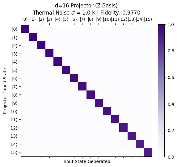
Z-Basis (Computational): The algorithm generates \(N\) standard basis states (e.g., \(|0\rangle, |1\rangle, \dots, |N-1\rangle\)). Physically, this means injecting a photon into exactly one waveguide at a time to test pure classical routing.
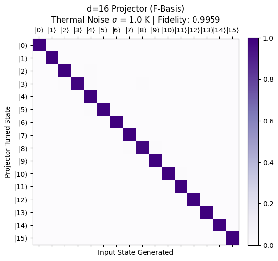
F-Basis (Fourier): The algorithm generates a Discrete Fourier Transform (DFT) matrix. Physically, these states represent complex quantum superpositions where the photon is smeared across all waveguides simultaneously with precise phase relationships. This is the ultimate stress test for the MZI network’s phase stability.
The Simulation Loop (
simulate_n_dimensional_basis):The script builds an \(N \times N\) probability matrix (a “confusion matrix”).
For every row, it tunes the chip to look for a specific target state using our reverse-propagation math (with thermal noise injected!).
For every column, it mathematical “injects” each possible input state and records the probability that the photon successfully reaches the target detector.
Fidelity and Visualization:
Because the chip has innate propagation losses, the raw probabilities are normalized so we measure the logical fidelity rather than the physical insertion loss.
The
fidelitymetric calculates how close the experimental matrix is to an ideal Identity matrix.Finally, it plots the results as a heatmap. A perfect system yields a solid, dark diagonal line (1.0 probability) with a pure white background (0.0 crosstalk). As thermal noise increases, you will see the fidelity drop and off-diagonal “dark counts” appear!
[5]:
z_states = [np.zeros(n_src, dtype=complex) for _ in range(n_src)]
for i in range(n_src): z_states[i][i] = 1.0

f_states = []
for l in range(n_src):
    state = np.zeros(n_src, dtype=complex)
    for k in range(n_src):
        state[k] = (1.0 / np.sqrt(n_src)) * np.exp(2j * np.pi * k * l / n_src)
    f_states.append(state)

def simulate_n_dimensional_basis(basis_states, basis_name, n_src, phase_offsets, temp_noise_std=0.0):
    probabilities = np.zeros((n_src, n_src))
    print(f"\n--- Simulating {n_src}D {basis_name}-Basis ---")

    for configured_idx, target_state in enumerate(basis_states):
        circuit_updates = get_tuning_for_measurement(target_state, phase_offsets, n_src, alice_tps_indices, alice_mzi_indices, temp_noise_std)
        s_matrix_circuit = projector_circuit.s_matrix(freqs, model_kwargs={"updates": circuit_updates})

        transfer_vector = np.array([
            s_matrix_circuit[(f"P{i}@0", target_port)][freq_idx] for i in range(n_src)
        ])

        for input_idx, input_state in enumerate(basis_states):
            amplitude = np.vdot(np.conj(transfer_vector), input_state)
            probabilities[configured_idx, input_idx] = np.abs(amplitude)**2

    max_prob = np.max(probabilities)
    normalized_probs = probabilities / max_prob
    fidelity = np.mean(np.sqrt(np.diag(normalized_probs)))

    fig, ax = plt.subplots(figsize=(6,6))
    cax = ax.matshow(normalized_probs, cmap='Purples', vmin=0, vmax=1)
    fig.colorbar(cax, fraction=0.046, pad=0.04)
    ax.set_xticks(range(n_src)); ax.set_yticks(range(n_src))
    ax.set_xticklabels([f'|{i}⟩' for i in range(n_src)])
    ax.set_yticklabels([f'|{i}⟩' for i in range(n_src)])
    ax.set_xlabel('Input State Generated')
    ax.set_ylabel('Projector Tuned State')
    ax.set_title(f'd={n_src} Projector ({basis_name}-Basis)\nThermal Noise $\\sigma$ = {temp_noise_std} K | Fidelity: {fidelity:.4f}')
    plt.show()


chip_phase_offsets = calibrate_phase_offsets(n_src, alice_mzi_indices)
simulate_n_dimensional_basis(z_states, "Z", n_src, chip_phase_offsets, temp_noise_std=noise_level)
simulate_n_dimensional_basis(f_states, "F", n_src, chip_phase_offsets, temp_noise_std=noise_level)
--- STEP 2: HARDWARE CALIBRATION (TARGET: P16) ---
P0 -> P16 | Transmission: 0.0295 | Phase Offset: 1.8983 rad
Progress: 100%
P1 -> P16 | Transmission: 0.0293 | Phase Offset: 0.9046 radProgress: 100%

P2 -> P16 | Transmission: 0.0290 | Phase Offset: -0.3068 radProgress: 100%

P3 -> P16 | Transmission: 0.0288 | Phase Offset: -1.3037 radProgress: 100%

P4 -> P16 | Transmission: 0.0285 | Phase Offset: -2.5171 radProgress: 100%

P5 -> P16 | Transmission: 0.0284 | Phase Offset: 2.7665 radProgress: 100%

P6 -> P16 | Transmission: 0.0282 | Phase Offset: 1.5544 radProgress: 100%

P7 -> P16 | Transmission: 0.0281 | Phase Offset: 0.5574 radProgress: 100%

P8 -> P16 | Transmission: 0.0279 | Phase Offset: -0.6566 radProgress: 100%

P9 -> P16 | Transmission: 0.0277 | Phase Offset: -1.6486 radProgress: 100%

P10 -> P16 | Transmission: 0.0274 | Phase Offset: -2.8644 rad
Progress: 100%
P11 -> P16 | Transmission: 0.0273 | Phase Offset: 2.4247 rad
Progress: 100%
P12 -> P16 | Transmission: 0.0271 | Phase Offset: 1.2071 rad
Progress: 100%
P13 -> P16 | Transmission: 0.0269 | Phase Offset: 0.2090 rad
Progress: 100%
P14 -> P16 | Transmission: 0.0268 | Phase Offset: -1.0052 radProgress: 100%

P15 -> P16 | Transmission: 0.0266 | Phase Offset: -2.0022 rad

--- Simulating 16D Z-Basis ---
Progress: 100%
Progress: 100%
Progress: 100%
Progress: 100%
Progress: 100%
Progress: 100%
Progress: 100%
Progress: 100%
Progress: 100%
Progress: 100%
Progress: 100%
Progress: 100%
Progress: 100%
Progress: 100%
Progress: 100%
Progress: 100%
Progress: 100%
--- Simulating 16D F-Basis ---
Progress: 100%
Progress: 100%
Progress: 100%
Progress: 100%
Progress: 100%
Progress: 100%
Progress: 100%
Progress: 100%
Progress: 100%
Progress: 100%
Progress: 100%
Progress: 100%
Progress: 100%
Progress: 100%
Progress: 100%
Progress: 100%