Analytic Waveguide Model

The AnalyticWaveguideModel provides a compact, physically meaningful description of 2-port waveguide components — straight waveguides, bends, and electro-optic (EO) phase shifters. It captures:

Feature	Parameters
Propagation	\(n_\text{eff}\), \(n_\text{group}\)
Dispersion	\(D\) (chromatic dispersion), \(S\) (dispersion slope)
Loss	\(L_p\) (propagation loss per unit length), \(L_0\) (extra loss, e.g. bend loss)
Temperature sensitivity	\(\mathrm{d}n/\mathrm{d}T\), \(\mathrm{d}L_p/\mathrm{d}T\)
Electro-optic modulation	\(V_{\pi L}\), \(\mathrm{d}L/\mathrm{d}V\), \(\mathrm{d}^2L/\mathrm{d}V^2\)

For each mode, the transmission between ports at frequency \(f\) is:

\[S_{12} = S_{21} = 10^{-L/20}\, e^{j(\beta\,\ell + \phi_{eo})}\]

where \(\ell\) is the waveguide length, \(\beta\) is a Taylor-expanded propagation constant around \(f_0\), and \(\phi_{eo} = \pi V \ell / V_{\pi L}\) is the electro-optic phase shift.

This notebook walks through the model parameter by parameter, building intuition with black_box_component before showing how to fit it to FDTD results on a real waveguide.

Setup

import matplotlib.pyplot as plt
import numpy as np
import photonforge as pf
import tidy3d as td

lossy_si = td.Medium.from_nk(n=3.475, k=1.4e-5, freq=pf.C_0 / 1.55)
tech = pf.basic_technology(core_medium=lossy_si, strip_width=0.5)
pf.config.default_technology = tech

wavelengths = np.linspace(1.5, 1.6, 101)
freqs = pf.C_0 / wavelengths

Basic Waveguide: Effective Index and Group Index

The simplest use of AnalyticWaveguideModel requires only n_eff. We use black_box_component to quickly create a test component without defining a physical layout.

The propagation constant is expanded as a Taylor series around the reference frequency \(f_0\):

\[\beta = \beta_0 + \beta_1\,\Delta\omega + \frac{\beta_2}{2}\,\Delta\omega^2 + \frac{\beta_3}{6}\,\Delta\omega^3\]

where \(\beta_0 = \omega_0\, n_\text{eff} / c_0\) and \(\beta_1 = n_\text{group} / c_0\). When n_group is not specified it defaults to n_eff, making the waveguide non-dispersive.

model_basic = pf.AnalyticWaveguideModel(
    n_eff=2.4,
    n_group=4.2,
    length=100,
)

bb_basic = model_basic.black_box_component(port_spec="Strip")
bb_basic

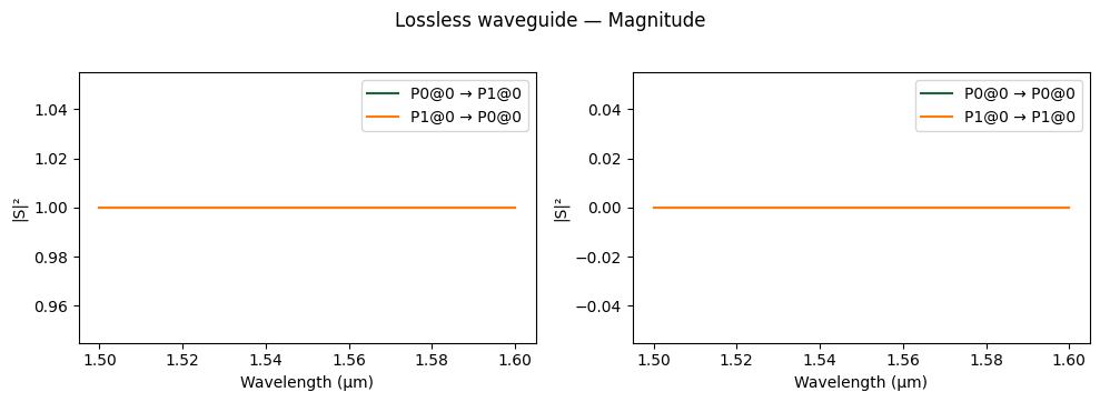
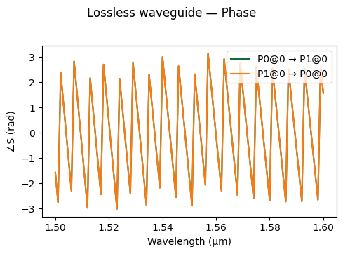
The S matrix of this lossless, dispersion-free waveguide has unit magnitude and a linearly varying phase:

s_basic = bb_basic.s_matrix(freqs)
pf.plot_s_matrix(s_basic)
plt.suptitle("Lossless waveguide — Magnitude", y=1.02)
plt.show()

Progress: 100%

pf.plot_s_matrix(s_basic, y="phase")
plt.suptitle("Lossless waveguide — Phase", y=1.02)
plt.show()

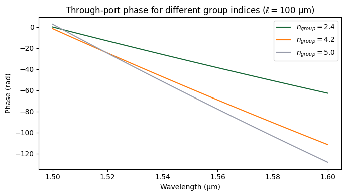
Effect of group index on phase slope

The group index \(n_\text{group}\) controls how rapidly the phase changes with frequency. A larger group index means a steeper phase slope. Below we compare three different group indices while keeping \(n_\text{eff}\) fixed.

port_names = sorted(s_basic.ports)
s_key = (f"{port_names[0]}@0", f"{port_names[1]}@0")

fig, ax = plt.subplots(figsize=(7, 4))
for ng in [2.4, 4.2, 5.0]:
    m = pf.AnalyticWaveguideModel(n_eff=2.4, n_group=ng, length=100)
    bb = m.black_box_component(port_spec="Strip")
    s = bb.s_matrix(freqs)
    pn = sorted(s.ports)
    key = (f"{pn[0]}@0", f"{pn[1]}@0")
    ax.plot(wavelengths, np.unwrap(np.angle(s[key])), label=f"$n_{{group}} = {ng}$")

ax.set_xlabel("Wavelength (µm)")
ax.set_ylabel("Phase (rad)")
ax.set_title("Through-port phase for different group indices ($\\ell = 100$ µm)")
ax.legend()
fig.tight_layout()
plt.show()

Progress: 100%
Progress: 100%
Progress: 100%

Chromatic Dispersion

Real waveguides exhibit chromatic dispersion: the group velocity varies with wavelength. The model captures this through the dispersion coefficient \(D\) and the dispersion slope \(S\):

\[\beta_2 = -\frac{\lambda_0}{\omega_0}\,D, \qquad \beta_3 = \left(\frac{\lambda_0}{\omega_0}\right)^2 \left(S + \frac{2}{\lambda_0}\,D\right)\]

Let’s compare a non-dispersive waveguide with two dispersive ones.

f0 = pf.C_0 / 1.55

fig, axes = plt.subplots(1, 2, figsize=(12, 4))

dispersions = [0, 2e-14, 4e-14]
labels = ["$D = 0$", "$D = 2 \\times 10^{-14}$", "$D = 4 \\times 10^{-14}$"]

for D, label in zip(dispersions, labels):
    m = pf.AnalyticWaveguideModel(
        n_eff=2.4,
        n_group=4.2,
        length=1000,
        dispersion=D,
        reference_frequency=f0,
    )
    bb = m.black_box_component(port_spec="Strip")
    s = bb.s_matrix(freqs)
    pn = sorted(s.ports)
    key = (f"{pn[0]}@0", f"{pn[1]}@0")
    phase = np.unwrap(np.angle(s[key]))

    axes[0].plot(wavelengths, np.abs(s[key]) ** 2, label=label)
    axes[1].plot(wavelengths, phase - phase[len(phase) // 2], label=label)

axes[0].set_xlabel("Wavelength (µm)")
axes[0].set_ylabel("$|S_{12}|^2$")
axes[0].set_title("Power (unchanged by dispersion)")
axes[0].legend()

axes[1].set_xlabel("Wavelength (µm)")
axes[1].set_ylabel("Phase − phase at centre (rad)")
axes[1].set_title("Phase curvature from dispersion ($\\ell = 1000$ µm)")
axes[1].legend()

fig.tight_layout()
plt.show()

Progress: 100%
Progress: 100%
Progress: 100%

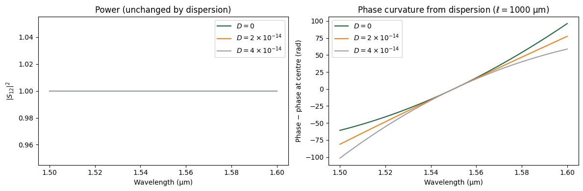
Dispersion does not change the transmitted power — it only curves the phase response. This matters in systems where precise phase relationships are needed (e.g. ring resonators, MZIs operating over a broad bandwidth).

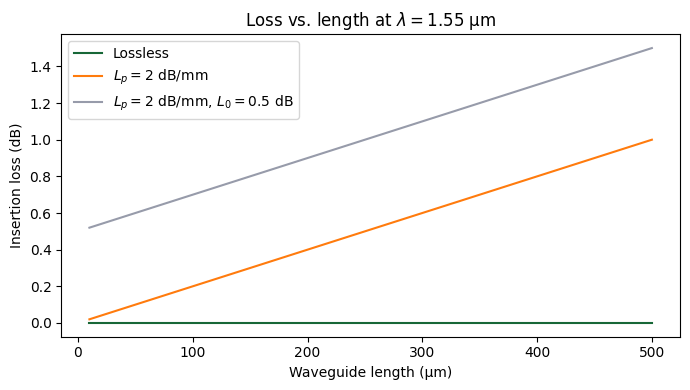
Loss: Propagation Loss and Extra Loss

The total loss in dB is:

\[L = L_0 + \ell\,L_p\]

• Propagation loss \(L_p\) (dB/µm): scales linearly with waveguide length — typical for scattering and absorption losses.

• Extra loss \(L_0\) (dB): a length-independent penalty, useful for modelling bend loss, mode-mismatch loss at junctions, etc.

Below we sweep waveguide length and compare the three cases.

f_center = np.array([pf.C_0 / 1.55])
lengths = np.linspace(10, 500, 5)

cases = [
    {"propagation_loss": 0.0,   "extra_loss": 0.0, "label": "Lossless"},
    {"propagation_loss": 2e-3,  "extra_loss": 0.0, "label": "$L_p = 2$ dB/mm"},
    {"propagation_loss": 2e-3,  "extra_loss": 0.5, "label": "$L_p = 2$ dB/mm, $L_0 = 0.5$ dB"},
]

fig, ax = plt.subplots(figsize=(7, 4))
for case in cases:
    insertion_loss = []
    for length in lengths:
        m = pf.AnalyticWaveguideModel(
            n_eff=2.4,
            n_group=4.2,
            length=length,
            propagation_loss=case["propagation_loss"],
            extra_loss=case["extra_loss"],
        )
        bb = m.black_box_component(port_spec="Strip")
        s = bb.s_matrix(f_center)
        pn = sorted(s.ports)
        key = (f"{pn[0]}@0", f"{pn[1]}@0")
        insertion_loss.append(-20 * np.log10(np.abs(s[key][0])))
    ax.plot(lengths, insertion_loss, label=case["label"])

ax.set_xlabel("Waveguide length (µm)")
ax.set_ylabel("Insertion loss (dB)")
ax.set_title("Loss vs. length at $\\lambda = 1.55$ µm")
ax.legend()
fig.tight_layout()
plt.show()

Progress: 100%
Progress: 100%
Progress: 100%
Progress: 100%
Progress: 100%
Progress: 100%
Progress: 100%
Progress: 100%
Progress: 100%
Progress: 100%
Progress: 100%
Progress: 100%
Progress: 100%
Progress: 100%
Progress: 100%

Temperature Sensitivity

The model accounts for temperature-dependent shifts in the effective index and propagation loss:

\[n_\text{eff}(T) = n_\text{eff}(T_0) + \frac{\mathrm{d}n_\text{eff}}{\mathrm{d}T}(T - T_0), \qquad L_p(T) = L_p(T_0) + \frac{\mathrm{d}L_p}{\mathrm{d}T}(T - T_0)\]

We will use the thermo-optic coefficient for bulk silicon (\(\mathrm{d}n/\mathrm{d}T \approx 1.8 \times 10^{-4}\;\text{K}^{-1}\)) as a rough approximation. Below we sweep temperature and observe the resulting phase shift.

T_ref = 293.0
temperatures = np.linspace(293, 353, 5)

fig, axes = plt.subplots(1, 2, figsize=(12, 4))

for T in temperatures:
    m = pf.AnalyticWaveguideModel(
        n_eff=2.4,
        n_group=4.2,
        length=200,
        dn_dT=1.8e-4,
        temperature=T,
        reference_temperature=T_ref,
        reference_frequency=f0,
    )
    bb = m.black_box_component(port_spec="Strip")
    s = bb.s_matrix(freqs)
    pn = sorted(s.ports)
    key = (f"{pn[0]}@0", f"{pn[1]}@0")
    axes[0].plot(wavelengths, np.abs(s[key]) ** 2, label=f"T = {T:.0f} K")
    axes[1].plot(wavelengths, np.unwrap(np.angle(s[key])), label=f"T = {T:.0f} K")

axes[0].set_xlabel("Wavelength (µm)")
axes[0].set_ylabel("$|S_{12}|^2$")
axes[0].set_title("Power (unchanged)")
axes[0].legend()

axes[1].set_xlabel("Wavelength (µm)")
axes[1].set_ylabel("Phase (rad)")
axes[1].set_title("Phase shift with temperature ($\\ell = 200$ µm)")
axes[1].legend()

fig.tight_layout()
plt.show()

Progress: 100%
Progress: 100%
Progress: 100%
Progress: 100%
Progress: 100%

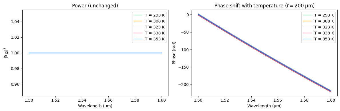
The power remains unchanged because dn_dT is real-valued here; a complex dn_dT would also shift the loss.

Electro-Optic Phase Shifter

The model supports EO modulation through three parameters:

• \(V_{\pi L}\): The voltage–length product (V·µm) required for a \(\pi\) phase shift. The EO phase is \(\phi_{eo} = \pi V \ell / V_{\pi L}\).

• \(\mathrm{d}L/\mathrm{d}V\): Linear voltage-dependent propagation loss (dB/µm/V).

• \(\mathrm{d}^2L/\mathrm{d}V^2\): Quadratic voltage-dependent propagation loss (dB/µm/V²).

When v_piL is set, the black_box_component automatically uses an EO phase-shifter thumbnail. Below we sweep the applied voltage and observe both phase shift and voltage-dependent loss.

length_eo = 500  # µm
v_piL = 10000  # V·µm → V_pi = 20 V for this length
v_pi = v_piL / length_eo

voltages = np.linspace(0, 2 * v_pi, 11)

phase_shift = []
insertion_loss_v = []

for V in voltages:
    m = pf.AnalyticWaveguideModel(
        n_eff=2.4,
        n_group=4.2,
        length=length_eo,
        propagation_loss=1e-3,
        v_piL=v_piL,
        dloss_dv=5e-5,
        voltage=V,
        reference_frequency=f0,
    )
    bb = m.black_box_component(port_spec="Strip")
    s = bb.s_matrix(f_center)
    pn = sorted(s.ports)
    key = (f"{pn[0]}@0", f"{pn[1]}@0")
    phase_shift.append(np.angle(s[key][0]))
    insertion_loss_v.append(-20 * np.log10(np.abs(s[key][0])))

phase_shift = np.unwrap(np.array(phase_shift))
phase_shift -= phase_shift[0]
insertion_loss_v = np.array(insertion_loss_v)

fig, axes = plt.subplots(1, 2, figsize=(12, 4))

ax = axes[0]
ax.plot(voltages, phase_shift / np.pi)
ax.axhline(1, color="C1", linestyle="--", alpha=0.6, label="$\\pi$ phase shift")
ax.axvline(v_pi, color="C2", linestyle=":", alpha=0.6, label=f"$V_\\pi = {v_pi:.0f}$ V")
ax.set_xlabel("Voltage (V)")
ax.set_ylabel("Phase shift ($\\pi$ rad)")
ax.set_title(f"EO phase shift ($\\ell = {length_eo}$ µm, $V_{{\\pi L}} = {v_piL}$ V·µm)")
ax.legend()

ax = axes[1]
ax.plot(voltages, insertion_loss_v)
ax.set_xlabel("Voltage (V)")
ax.set_ylabel("Insertion loss (dB)")
ax.set_title("Voltage-dependent loss (dL/dV = $5 \\times 10^{-5}$ dB/µm/V)")

fig.tight_layout()
plt.show()

Progress: 100%
Progress: 100%
Progress: 100%
Progress: 100%
Progress: 100%
Progress: 100%
Progress: 100%
Progress: 100%
Progress: 100%
Progress: 100%
Progress: 100%

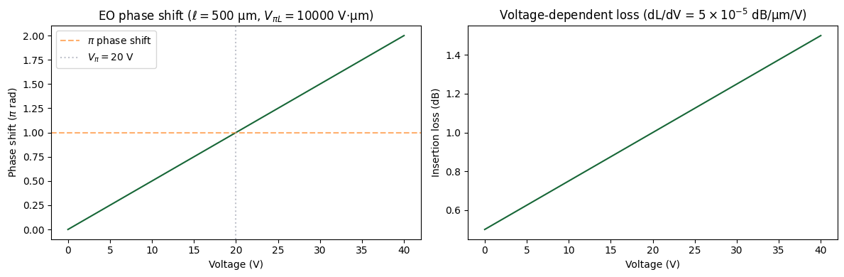
The phase increases linearly with voltage, reaching \(\pi\) at \(V_\pi = V_{\pi L} / \ell\). The insertion loss also increases with voltage due to the carrier-induced absorption captured by dloss_dv.

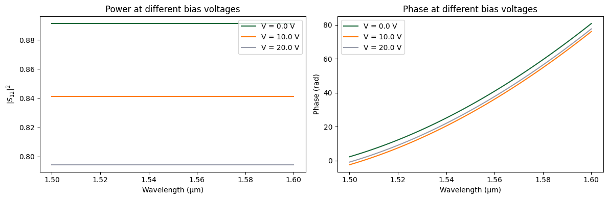
Spectral view at different bias voltages

The voltage parameter can be passed to s_matrix via model_kwargs to override the model default, which is convenient for voltage sweeps without re-creating the model.

model_eo = pf.AnalyticWaveguideModel(
    n_eff=2.4,
    n_group=4.2,
    length=length_eo,
    propagation_loss=1e-3,
    v_piL=v_piL,
    dloss_dv=5e-5,
    reference_frequency=f0,
)
bb_eo = model_eo.black_box_component(port_spec="Strip")

fig, axes = plt.subplots(1, 2, figsize=(12, 4))
for V in [0, v_pi / 2, v_pi]:
    s = bb_eo.s_matrix(freqs, model_kwargs={"voltage": V})
    pn = sorted(s.ports)
    key = (f"{pn[0]}@0", f"{pn[1]}@0")
    axes[0].plot(wavelengths, np.abs(s[key]) ** 2, label=f"V = {V:.1f} V")
    axes[1].plot(wavelengths, np.unwrap(np.angle(s[key])), label=f"V = {V:.1f} V")

axes[0].set_xlabel("Wavelength (µm)")
axes[0].set_ylabel("$|S_{12}|^2$")
axes[0].set_title("Power at different bias voltages")
axes[0].legend()

axes[1].set_xlabel("Wavelength (µm)")
axes[1].set_ylabel("Phase (rad)")
axes[1].set_title("Phase at different bias voltages")
axes[1].legend()

fig.tight_layout()
plt.show()

Progress: 100%
Progress: 100%
Progress: 100%