Chip Simulation

This notebook details the simulation phase of the tutorial series. Building upon the physical parameters and component libraries established in preceding notebooks, we will now simulate the functional performance of the designed Photonic Integrated Circuit (PIC) in both the frequency and time domains using PhotonForge.

Operational Principles of the Transmitter

The device under test is a 4-channel Wavelength Division Multiplexing (WDM) transmitter. Its core operation is defined by the following subsystems:

• Modulation Core: Each individual channel utilizes a Mach-Zehnder Modulator (MZM) driven by a dual-arm electro-optic (EO) phase shifter. This architecture facilitates the encoding of high-speed electrical data onto a continuous optical carrier wave.

• Thermo-Optic Biasing: To ensure each MZM operates accurately at its optimal quadrature (3dB) point, thermo-optic phase shifters (micro-heaters) are integrated into the design. Precise thermal tuning allows us to adjust the optical phase and stabilize the required operational bias.

• Multiplexing: The circuit is designed to process four distinct wavelength channels, ranging from approximately 1548 nm to 1556 nm. Following modulation, an optical multiplexer combines these four independent signals into a single output waveguide.

Simulation Methodology

To accurately model the performance of this system, our workflow will follow these sequential phases:

1. DC Biasing Calculation: Analytically calculate the requisite temperature for each micro-heater to achieve the target 3dB transmission bias at its respective operating wavelength.

2. Frequency-Domain Analysis: Evaluate the scattering matrix (S-parameters) of both the individual components and the fully multiplexed PIC to verify static transmission behavior and calculate insertion losses.

3. Time-Domain Stepping: Utilize the SMatrixTimeStepper to simulate dynamic operation by injecting pseudo-random electrical bit sequences into the MZMs alongside Continuous Wave (CW) optical inputs.

4. Transient Response Extraction: Extract and plot the time-domain output optical power relative to the electrical drive voltage to validate the dynamic signal integrity of each channel.

%%capture
# Load building blocks defined earlier.
# Expected symbols used below include (names as defined in `Chip_Layout.ipynb`):
# - `ps`: dual-arm EO phase-shifter (modulator core)
# - `heater`: thermo-optic phase shifter (used here for trimming)
# - `single_modulator_block`, `mux_block`: functions to generate our sub-circuits
# - `pic`: the fully assembled 4-channel transmitter circuit
# - `n_eff`, `n_group`, `n_eff_rib`, `n_group_rib`, `propagation_loss`, `freq0`: waveguide parameters
# - `wavelengths`, `lambda0`: operational wavelength definitions
%run Chip_Layout.ipynb

Progress: 100%
Progress: 100%
Progress: 100%
Progress: 100%
Progress: 100%
Progress: 100%
Progress: 100%
Progress: 100%
Progress: 100%
Progress: 100%
Progress: 100%
Progress: 100%
Progress: 100%
Progress: 100%

viewer = LiveViewer()

LiveViewer started at http://localhost:40653

Waveguide Modeling and Simulation Parameters

To ensure the simulation accurately reflects physical chip performance, we apply an analytic waveguide model to all routing components (straights, bends, and S-bends). This model explicitly accounts for realistic propagation losses and dispersion (via effective and group indices) arising from fabrication imperfections.

Additionally, we configure the default SMatrixTimeStepper with a slightly increased RMS error tolerance. This optimizes the dynamic simulation performance and suppresses unnecessary runtime warnings.

# Define an analytic waveguide model to simulate realistic on-chip optical propagation,
# explicitly accounting for propagation losses due to fabrication imperfections.
wg_model = pf.AnalyticWaveguideModel(
    n_eff=n_eff,
    reference_frequency=freq0,
    propagation_loss=propagation_loss,
    n_group=n_group,
)

# Apply this realistic model globally to all routing components.
pf.config.default_kwargs["bend"] = {"model": wg_model}
pf.config.default_kwargs["s_bend"] = {"model": wg_model}
pf.config.default_kwargs["straight"] = {"model": wg_model}

# Set the RMS error tolerance for the default SMatrixTimeStepper.
# Increased slightly to avoid runtime warnings during dynamic simulation.
from photonforge import SMatrixTimeStepper
pf.config.default_time_steppers['*'] = SMatrixTimeStepper(rms_error_tolerance=0.001)

DC Biasing: Analytic Temperature Calculation

To operate the Mach-Zehnder Modulators at their optimal region of linearity (the quadrature or 3dB point), a static optical phase shift must be applied to one of the modulator arms. This is achieved by trimming the integrated thermo-optic micro-heaters.

The following cell defines a core helper function, get_bias_temperature, which calculates the precise heater temperature required to achieve a target transmission drop (defaulting to a 3.0 dB bias). Because calculating this through brute-force simulation would be computationally expensive, this function uses an analytic approach:

1. Baseline Extraction: Evaluates the unbiased transmission of the MZM at ambient temperature (293 K).

2. Phase Calculation: Derives the necessary phase difference required to hit the target transmission power.

3. Thermo-Optic Conversion: Converts the candidate optical phase shifts into required temperature deltas (\(\Delta T\)) using the waveguide’s thermo-optic coefficient (dn_dT).

4. Validation: Iterates through the calculated candidates and returns the minimum physical temperature (strictly greater than 293 K) that satisfies the biasing condition within an acceptable tolerance.

def get_bias_temperature(
    heater_kwargs,
    single_modulator,
    heater_name,
    wavelengths,
    target_wavelength,
    bias_dB=3.0,
    port_in="P0@0",
    port_out="P1@0",
):
    """
    Analytically calculates candidate heater temperatures to bias an MZM,
    and returns the minimum temperature strictly > 293 K that yields the target.
    """
    # 1. Determine baseline and target transmission power
    baseline_s_matrix = single_modulator.s_matrix(pf.C_0 / wavelengths)
    t_power_baseline = np.abs(baseline_s_matrix[(port_in, port_out)]) ** 2
    t_max = np.max(t_power_baseline)
    target_t_power = t_max * (10 ** (-bias_dB / 10.0))

    # Interpolate in the wavelength domain (assumes wavelengths array is increasing)
    t_curr = np.interp(target_wavelength, wavelengths, t_power_baseline)

    # 2. Extract parameters
    length = heater_kwargs["length"]
    current_temp = heater_kwargs["temperature"]  # Baseline: 293.0 K
    dn_dT = np.asarray(heater_kwargs["dn_dT"]).item()

    # 3. Calculate absolute phases [0, pi]
    phi_curr = 2 * np.arccos(np.clip(np.sqrt(t_curr / t_max), 0.0, 1.0))
    phi_target = 2 * np.arccos(np.clip(np.sqrt(target_t_power / t_max), 0.0, 1.0))

    # 4. Generate the 4 possible positive phase shifts
    two_pi = 2 * np.pi
    candidates_phi = [
        (phi_target - phi_curr) % two_pi,
        (-phi_target - phi_curr) % two_pi,
        (phi_target - (-phi_curr)) % two_pi,
        (-phi_target - (-phi_curr)) % two_pi,
    ]

    # 5. Convert phase candidates to Delta T candidates
    # Using target_wavelength directly (since it is already in um)
    phase_to_temp_factor = target_wavelength / (two_pi * dn_dT * length)

    candidates_dT = []
    for phi in set(candidates_phi):
        # If the shift is effectively 0, push it to the next cycle
        # to guarantee the temperature increases strictly > 293.0
        if phi < 1e-4:
            phi += two_pi
        candidates_dT.append(phi * phase_to_temp_factor)

    # Sort from smallest temperature shift to largest
    candidates_dT.sort()

    # 6. Test candidates and select the smallest valid temperature
    tested_temps = []

    # Convert wavelengths to frequencies for the PhotonForge S-matrix solver
    freqs = pf.C_0 / wavelengths

    for dT in candidates_dT:
        test_temp = current_temp + dT

        # Evaluate transmission at test_temp
        updates = {(heater_name, 0): {"model_updates": {"temperature": test_temp}}}
        s_mat = single_modulator.s_matrix(freqs, model_kwargs={"updates": updates})

        # Interpolate test results in the wavelength domain
        t_test_array = np.abs(s_mat[(port_in, port_out)]) ** 2
        t_test = np.interp(target_wavelength, wavelengths, t_test_array)

        error = np.abs(t_test - target_t_power)
        tested_temps.append((test_temp, error))

        # Because we sorted ascending, the first one to hit the target
        # (within a 2% linear power tolerance) is our minimum valid temperature.
        if error < 0.02 * t_max:
            return test_temp

    # Fallback: if the MZM is highly non-ideal and no candidate was perfect,
    # return the tested temperature that got us the closest to the target.
    tested_temps.sort(key=lambda x: x[1])
    return tested_temps[0][0]

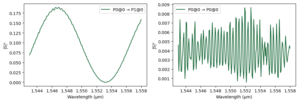
With the analytic biasing algorithm established, we will now apply it to a standalone Mach-Zehnder Modulator. This step serves to validate the thermo-optic trimming process before scaling it to the full 4-channel multiplexed circuit.

We will calculate the necessary heater temperature to achieve a 3.0 dB transmission bias at the primary reference wavelength (lambda0). This computed temperature is then injected into the component model via an updates dictionary. Finally, we compute and plot the frequency-domain scattering matrix (S-matrix) to visually confirm the transmission spectrum and verify that the bias point has been accurately set.

# Instantiate a single MZM sub-circuit for testing
single_modulator = single_modulator_block()
viewer(single_modulator)

# Calculate the precise temperature required to achieve a 3 dB bias at lambda0
bias_temp = get_bias_temperature(
    heater_kwargs=heater.active_model.parametric_kwargs,
    single_modulator=single_modulator,
    heater_name=heater.name,
    wavelengths=wavelengths,
    target_wavelength=lambda0,
    bias_dB=3.0,
)

# Package the computed temperature into an updates dictionary.
# This structure targets the specific heater instance within the modulator model.
updates = {(heater.name, 0): {"model_updates": {"temperature": bias_temp}}}

# Compute the static S-matrix across the frequency grid using the updated heater temperature
s_matrix_mod = single_modulator.s_matrix(freqs, model_kwargs={"updates": updates})

# Plot the transmission spectrum from the input port (P0) to visually verify the bias point
_ = pf.plot_s_matrix(s_matrix_mod, input_ports=["P0"])

Starting…

10:04:09 EDT Loading simulation from local cache. View cached task using web UI
             at
             'https://tidy3d.simulation.cloud/workbench?taskId=fdve-d259da32-c52
             0-456f-9f87-869e22017cbd'.

             Loading simulation from local cache. View cached task using web UI
             at
             'https://tidy3d.simulation.cloud/workbench?taskId=fdve-2163548d-126
             c-43ec-a92a-b42a76307dc7'.

Progress: 100%
Progress: 100%
Progress: 100%

Time-Domain Simulation: Single Modulator

Having verified the static biasing of the standalone Mach-Zehnder Modulator, we now shift our focus to dynamic time-domain simulation. To evaluate the transient response and signal integrity of the modulator, we must generate appropriate high-speed electrical and optical stimuli.

The following cell establishes the simulation time grid and synthesizes a pseudo-random binary sequence (PRBS). This digital sequence is upsampled and converted into an analog wave amplitude, normalized to a standard 50-ohm characteristic impedance. Because the dual-arm phase shifter operates in a push-pull configuration, we generate complementary electrical drive signals to drive the two modulator arms differentially.

Simultaneously, a constant Continuous Wave (CW) optical input is defined to act as the carrier signal. These individual waveforms are subsequently bundled into a TimeSeries object, which will serve as the standardized input vector for our time-domain solver.

# Define the fundamental time grid parameters
bit_rate = 10e9
samples_per_bit = 200
n_bits = 20

# Generate the discrete time vector based on the required resolution per bit
time_step = 1.0 / (bit_rate * samples_per_bit)
N_steps = int(n_bits * samples_per_bit)
t = time_step * np.arange(N_steps)

# Generate a pseudo-random bit sequence (PRBS) of 0s and 1s
np.random.seed(1)
bits = np.random.randint(0, 2, n_bits)

# Upsample the digital bits to the simulation time grid and convert to wave amplitude.
# The amplitude is scaled assuming a characteristic impedance (Z0) of 50 ohms.
Z0 = 50
E0_in = 2 * (np.repeat(bits, samples_per_bit) - 0.5) / (Z0**0.5)

# Define a Continuous Wave (CW) optical carrier signal at the input port
Opt_in = np.ones(len(t))

# Bundle the localized waveforms into a PhotonForge TimeSeries object.
# Note the complementary push-pull electrical drive applied to E0 and E1.
inputs_mod = pf.TimeSeries(
    values={
        "E0@0": E0_in,   # Electrical drive for the first modulator arm
        "E1@0": -E0_in,  # Complementary electrical drive for the second arm
        "P0@0": Opt_in,  # CW optical carrier input
    },
    time_step=time_step,
)

With the input stimuli defined, we can proceed to simulate the transient response of the single modulator. Before executing the run, we calculate the dispersion-adjusted effective index at the specific carrier frequency to ensure phase accuracy in the time domain. This will be passed to phase modulator’s time stepper. The setup_time_stepper method is then initialized, incorporating our previously calculated static heater bias. Finally, we execute the simulation using our synthesized input waveforms.

# Carrier frequency
f_c = pf.C_0/lambda0

# Calculate the updated n_eff_rib at the carrier frequency
n_eff_rib_fc = n_eff_rib + (n_group_rib - n_eff_rib) * (f_c - freq0) / freq0
ps.update(ref_freq=f_c, n_eff=n_eff_rib_fc)


# Build time-stepper (frequency grid used internally for fitting/conversion)
ts_mod = single_modulator.setup_time_stepper(
    time_step=time_step,
    carrier_frequency=f_c,
    time_stepper_kwargs={
        "frequencies": freqs,
        "updates": updates,
    },
)

# Run
outputs = ts_mod.step(inputs_mod)

10:04:19 EDT Loading simulation from local cache. View cached task using web UI
             at
             'https://tidy3d.simulation.cloud/workbench?taskId=mo-f3052792-1091-
             4dc8-9dd0-ce349ed99f52'.

             Loading simulation from local cache. View cached task using web UI
             at
             'https://tidy3d.simulation.cloud/workbench?taskId=mo-de800ba0-e169-
             42de-9ca0-275262e95b6f'.

10:04:21 EDT Loading simulation from local cache. View cached task using web UI
             at
             'https://tidy3d.simulation.cloud/workbench?taskId=mo-c667a717-507b-
             4c8a-8da7-85f4b56b2fe9'.

             Loading simulation from local cache. View cached task using web UI
             at
             'https://tidy3d.simulation.cloud/workbench?taskId=mo-3567a091-50e9-
             418c-9d38-e566198c9e82'.

10:04:22 EDT Loading simulation from local cache. View cached task using web UI
             at
             'https://tidy3d.simulation.cloud/workbench?taskId=mo-fa7a7c2e-d520-
             4faf-8e2c-c4b1663f963c'.

             Loading simulation from local cache. View cached task using web UI
             at
             'https://tidy3d.simulation.cloud/workbench?taskId=mo-818f1faf-7a4e-
             4b3c-b298-9b24a5c2dbb8'.

Progress: 100%
Progress: 4000/4000

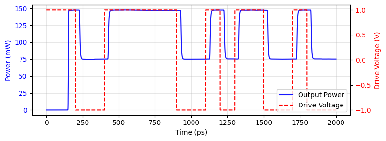
The generated plot visualizes the time-domain performance of the single modulator, revealing two key behavioral characteristics:

1. Propagation Delays: The optical output power begins to appear only after an initial absolute delay, which corresponds to the optical transit time through the entire physical length of the Mach-Zehnder Interferometer (MZI) structure. Once the optical signal emerges, it closely tracks the applied electrical drive voltage, subject only to a minor secondary delay dictated by the length of the active modulator section.

2. Extinction Ratio Verification: This result directly validates our initial component design. As specified in the Component Library notebook, the modulator was engineered to yield a 3 dB extinction ratio when driven by a 2 Vpp signal at a quadrature bias point. The transient waveform clearly demonstrates this expected dynamic range, confirming both the layout and the applied DC thermal bias.

p_out = np.abs(outputs["P1@0"]) ** 2

fig, ax1 = plt.subplots(figsize=(8, 3))

# Plot Output Power on the primary y-axis (left)
ax1.plot(t * 1e12, p_out * 1e3, color='blue', label="Output Power", alpha=0.9)
ax1.set_xlabel("Time (ps)")
ax1.set_ylabel("Power (mW)", color='blue')
ax1.tick_params(axis='y', labelcolor='blue')
ax1.grid(True, alpha=0.3)

# Create a twin axis for the Electrical Drive (right)
ax2 = ax1.twinx()
ax2.plot(t * 1e12, E0_in * Z0 ** 0.5, color='red', label="Drive Voltage", linestyle='--')
ax2.set_ylabel("Drive Voltage (V)", color='red')
ax2.tick_params(axis='y', labelcolor='red')

# Combine legends from both axes
lines1, labels1 = ax1.get_legend_handles_labels()
lines2, labels2 = ax2.get_legend_handles_labels()
ax2.legend(lines1 + lines2, labels1 + labels2,loc='lower right')

plt.tight_layout()
plt.show()

Multiplexer Characterization and Channel Identification

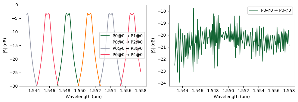
Before simulating the fully assembled 4-channel transmitter, it is necessary to characterize the standalone optical multiplexer. The multiplexer is responsible for combining the four modulated optical signals into a single output waveguide.

By computing and plotting the frequency-domain scattering matrix of the multiplexer, we can visualize its transmission spectrum and clearly identify the passbands. From the resulting plot, we will extract the exact center wavelengths corresponding to the peak transmission of each channel. These identified wavelengths are critical, as they will serve as the targeted operational carrier frequencies (ldas) for biasing and driving the respective modulators in the full circuit simulation.

# Instantiate the optical multiplexer sub-circuit
mux = mux_block()
viewer(mux)

# Compute the static S-matrix across the defined frequency grid
s_matrix_mux = mux.s_matrix(freqs)

# Plot the transmission spectrum (in dB) from the input ports
# This allows us to visually identify the transmission peaks for each channel
fig, axes = pf.plot_s_matrix(s_matrix_mux, y='dB', input_ports=["P0"])

# Restrict the y-axis range to focus on the relevant passband features
axes[0].set_ylim(-30, 0)

Progress: 100%

(-30.0, 0.0)

# Define the center wavelengths (in micrometers) extracted from the multiplexer transmission plot.
ldas = [1.5484, 1.5512, 1.5540, 1.5568]

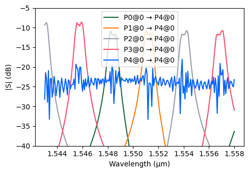
Full Circuit Static Analysis (Unbiased)

Having characterized the individual building blocks, we now transition to evaluating the fully assembled 4-channel transmitter. In our circuit architecture, ports P0 through P3 are designated as the individual optical inputs for the four distinct wavelength channels, while port P4 serves as the combined, multiplexed output.

The following cell calculates and plots the frequency-domain scattering matrix of the complete Photonic Integrated Circuit (PIC) at ambient conditions—prior to applying any thermo-optic biasing to the modulators. By filtering the plot to specifically display the transmission reaching the output port (P4), we can observe the raw passbands, baseline insertion losses, and outputs at different bias points because of the uncalibrated system.

viewer(pic)

s_matrix_chip = pic.s_matrix(freqs)
fig, axes = pf.plot_s_matrix(s_matrix_chip, y="dB", output_ports=["P4"], threshold=0)
axes[0].set_ylim(-30, -5)

Starting…

10:04:47 EDT Loading simulation from local cache. View cached task using web UI
             at
             'https://tidy3d.simulation.cloud/workbench?taskId=fdve-42dd90db-5ee
             d-4a75-aa14-f9e0f1a0519f'.

             Loading simulation from local cache. View cached task using web UI
             at
             'https://tidy3d.simulation.cloud/workbench?taskId=fdve-0f7e6eae-efd
             9-414f-87aa-83cc432805ad'.

10:04:49 EDT Loading simulation from local cache. View cached task using web UI
             at
             'https://tidy3d.simulation.cloud/workbench?taskId=mo-b0b5d759-09c5-
             4b90-a734-b60a40e19f42'.

10:04:54 EDT Loading simulation from local cache. View cached task using web UI
             at
             'https://tidy3d.simulation.cloud/workbench?taskId=fdve-acdd74de-3bf
             d-47bc-996b-70f7bf780b07'.

10:04:55 EDT Loading simulation from local cache. View cached task using web UI
             at
             'https://tidy3d.simulation.cloud/workbench?taskId=fdve-7e892e39-c1d
             5-4eb6-a033-9d0759f30483'.

10:05:01 EDT Loading simulation from local cache. View cached task using web UI
             at
             'https://tidy3d.simulation.cloud/workbench?taskId=fdve-f9bcfc13-466
             a-4cbd-b5d9-b8abef4a7c0b'.

10:05:02 EDT Loading simulation from local cache. View cached task using web UI
             at
             'https://tidy3d.simulation.cloud/workbench?taskId=fdve-eb8fe9ab-be8
             f-43fd-beb3-15603bcda92b'.

10:05:07 EDT Loading simulation from local cache. View cached task using web UI
             at
             'https://tidy3d.simulation.cloud/workbench?taskId=fdve-8c019b2c-7a3
             d-48f9-a247-a6d275d37f83'.

10:05:08 EDT Loading simulation from local cache. View cached task using web UI
             at
             'https://tidy3d.simulation.cloud/workbench?taskId=fdve-ca2e5edd-fb2
             4-42eb-b7ae-e43e6060dc51'.

10:05:14 EDT Loading simulation from local cache. View cached task using web UI
             at
             'https://tidy3d.simulation.cloud/workbench?taskId=fdve-b2283074-d2c
             5-4936-9ea5-ecd933222e2e'.

10:05:15 EDT Loading simulation from local cache. View cached task using web UI
             at
             'https://tidy3d.simulation.cloud/workbench?taskId=fdve-25204c6f-79c
             9-486e-a1f1-bed5c3c1b3dd'.

Progress: 100%

(-30.0, -5.0)

Full Circuit Biasing: 4-Channel Calibration

Having established the exact center wavelengths for our four channels (ldas), we must now calibrate the entire multiplexed circuit. Because each Mach-Zehnder Modulator operates at a different carrier wavelength, the exact temperature required to induce a \(3\text{ dB}\) optical phase shift will vary slightly from channel to channel due to wavelength-dependent dispersion.

The following cell automates this calibration process. It iterates through the four modulator instances within the assembled Photonic Integrated Circuit (PIC), calculating the unique bias temperature required for each specific channel. Finally, it constructs a hierarchical updates dictionary. This dictionary maps the calculated thermal biases to the exact heater components buried within the nested circuit structure, ensuring each modulator is perfectly tuned for its respective data stream.

# Initialize an empty dictionary to store the thermal biases for the time-stepper
updates = {}

# Iterate through the 4 independent channels of the transmitter
for i in range(4):
    # Extract the individual modulator component reference directly from the PIC
    mod_component = pic.references[i].component

    # Calculate the required heater temperature to achieve a 3.0 dB bias
    # using the specific target_wavelength (ldas[i]) for this channel.
    bias_temp = get_bias_temperature(
        heater_kwargs=heater.active_model.parametric_kwargs,
        single_modulator=mod_component,
        heater_name=heater.name,
        wavelengths=wavelengths,
        target_wavelength=ldas[i],
        bias_dB=3.0,
    )

    # The key is a tuple defining the path: (modulator_name, modulator_instance, heater_name, heater_instance)
    updates[(mod_component.name, 0, heater.name, 0)] = {"model_updates": {"temperature": bias_temp}}

Starting…

10:05:22 EDT Loading simulation from local cache. View cached task using web UI
             at
             'https://tidy3d.simulation.cloud/workbench?taskId=fdve-4419de4c-8ff
             8-406e-abb7-243694d22384'.

             Loading simulation from local cache. View cached task using web UI
             at
             'https://tidy3d.simulation.cloud/workbench?taskId=fdve-145b985b-e3b
             6-4f33-9e6a-4b194c63fd2b'.

Progress: 100%
Progress: 100%
Progress: 100%
Progress: 100%
Progress: 100%
Progress: 100%
Progress: 100%
Progress: 100%
Progress: 100%
Progress: 100%

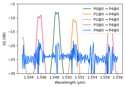
With the hierarchical updates dictionary now populated with the calibrated thermal biases for all four channels, we will recalculate the static scattering matrix of the fully assembled transmitter.

By plotting the transmission to the multiplexed output port (P4), we can visually verify the success of the calibration process. The resulting spectrum should demonstrate that all four channels achieve nearly identical transmission levels at their respective center wavelengths (ldas). This uniform response confirms that the target 3 dB bias has been correctly and independently established for each Mach-Zehnder Modulator, effectively compensating for wavelength-dependent dispersion.

s_matrix_chip_3dB = pic.s_matrix(freqs, model_kwargs={"updates": updates})
fig, axes = pf.plot_s_matrix(s_matrix_chip_3dB, y="dB", output_ports=["P4"], threshold=0)
axes[0].set_ylim(-40, -5)

Progress: 100%

(-40.0, -5.0)

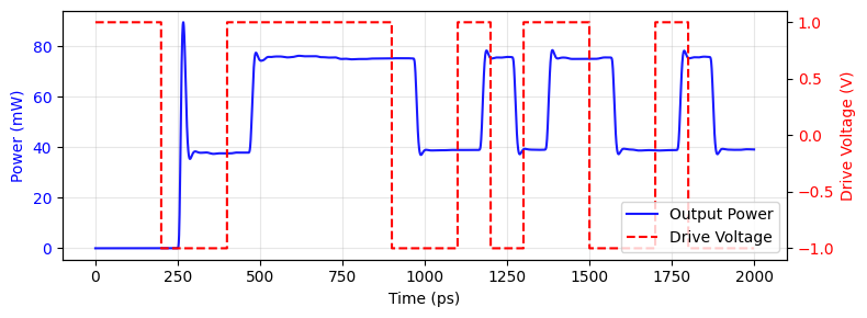
Dynamic Simulation: Full Circuit (Channel 1)

With the complete 4-channel transmitter properly biased, we can now evaluate its dynamic time-domain performance. We will test the data transmission sequentially, beginning with the first channel.

To isolate the response of Channel 1, we direct our synthesized Continuous Wave (CW) optical carrier specifically into the first input port (P0) and apply the high-speed electrical drive signals to the corresponding modulator arms (E0 and E1).

Crucially, the time-stepper is configured to operate at the exact center wavelength previously identified for this specific channel. By applying the comprehensive updates dictionary to the solver, we ensure the entire circuit - including all four micro-heaters - remains correctly thermally biased as the transient signals propagate toward the multiplexed output port.

# We specifically target Channel 1 by injecting the optical carrier into P0
# and driving its corresponding modulator via electrical ports E0 and E1.
inputs_pic = pf.TimeSeries(
    values={
        "E0@0": E0_in,
        "E1@0": -E0_in,
        "P0@0": Opt_in,
    },
    time_step=time_step,
)

# Define the optical carrier frequency explicitly for Channel 1's center wavelength
f_c = pf.C_0 / ldas[0]

# Update the phase shifter's effective index to account for linear dispersion
n_eff_rib_fc = n_eff_rib + (n_group_rib - n_eff_rib) * (f_c - freq0) / freq0
ps.update(ref_freq=f_c, n_eff=n_eff_rib_fc)

# Initialize the time-stepper for the fully assembled PIC.
# We pass the comprehensive 'updates' dictionary to ensure all 4 modulators
ts_pic = pic.setup_time_stepper(
    time_step=time_step,
    carrier_frequency=f_c,
    time_stepper_kwargs={
        "frequencies": freqs,
        "updates": updates,
    },
)

outputs = ts_pic.step(inputs_pic)

10:06:25 EDT Loading simulation from local cache. View cached task using web UI
             at
             'https://tidy3d.simulation.cloud/workbench?taskId=mo-6f96886f-bf29-
             461c-8d61-21c1e08402ad'.

             Loading simulation from local cache. View cached task using web UI
             at
             'https://tidy3d.simulation.cloud/workbench?taskId=mo-9f147dfe-a065-
             456e-9949-5bc3b86acf8d'.

10:06:27 EDT Loading simulation from local cache. View cached task using web UI
             at
             'https://tidy3d.simulation.cloud/workbench?taskId=mo-7e87bf7f-a64e-
             479b-86fb-24df53088df4'.

             Loading simulation from local cache. View cached task using web UI
             at
             'https://tidy3d.simulation.cloud/workbench?taskId=mo-6a09810c-efb8-
             4916-8de0-81ec7a1ded07'.

10:06:28 EDT Loading simulation from local cache. View cached task using web UI
             at
             'https://tidy3d.simulation.cloud/workbench?taskId=mo-27949552-26f9-
             462b-baf5-f73c2893d627'.

             Loading simulation from local cache. View cached task using web UI
             at
             'https://tidy3d.simulation.cloud/workbench?taskId=mo-dbfb4422-02fc-
             493e-9c55-02520b81cbb1'.

Progress: 100%
Progress: 4000/4000

The resulting plot visualizes the time-domain output of the first multiplexed channel at the final output port (P4). Comparing this waveform to the standalone modulator simulated earlier, three key differences emerge:

1. Increased Propagation Delay: The optical signal exhibits a significantly longer absolute delay before appearing at the output. This accounts for the extended physical transit time through the entire input routing, the Mach-Zehnder Interferometer, the output routing, and finally, the multiplexer.

2. Increased Insertion Loss: The peak absolute optical power is noticeably lower. This expected drop is due to the combined insertion losses of the optical multiplexer and the additional physical waveguide routing across the chip.

3. Extinction Ratio Degradation: While the extinction ratio remains approximately 3 dB, it is slightly degraded compared to the ideal standalone component. This is a realistic consequence of signal propagation through a cascaded optical system, where frequency-dependent behavior (dispersion) and the filtering effects of the multiplexer passband slightly distort the broadband modulated signal.

p_out = np.abs(outputs["P4@0"]) ** 2

fig, ax1 = plt.subplots(figsize=(8, 3))

# Plot Output Power on the primary y-axis (left)
ax1.plot(t * 1e12, p_out * 1e3, color='blue', label="Output Power", alpha=0.9)
ax1.set_xlabel("Time (ps)")
ax1.set_ylabel("Power (mW)", color='blue')
ax1.tick_params(axis='y', labelcolor='blue')
ax1.grid(True, alpha=0.3)

# Create a twin axis for the Electrical Drive (right)
ax2 = ax1.twinx()
ax2.plot(t * 1e12, E0_in  * Z0 ** 0.5, color='red', label="Drive Voltage", linestyle='--')
ax2.set_ylabel("Drive Voltage (V)", color='red')
ax2.tick_params(axis='y', labelcolor='red')

# Combine legends from both axes
lines1, labels1 = ax1.get_legend_handles_labels()
lines2, labels2 = ax2.get_legend_handles_labels()
ax2.legend(lines1 + lines2, labels1 + labels2,loc='lower right')

plt.tight_layout()
plt.show()

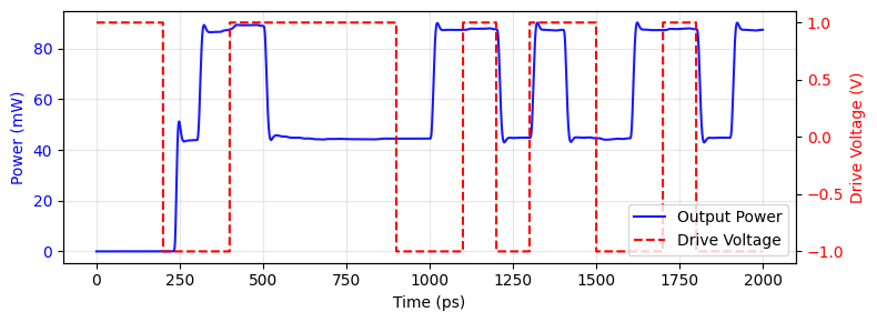
Dynamic Simulation: Full Circuit (Channel 4)

To confirm consistent dynamic performance across the transmitter’s entire operating bandwidth, we conclude by evaluating the fourth and final multiplexed channel.

The procedure perfectly mirrors the approach used for Channel 1. However, to isolate Channel 4, we direct the Continuous Wave (CW) optical carrier into input port P3 and apply the differential electrical drive to its specific modulator arms (ports E6 and E7). The time-stepper is updated to operate at the target center wavelength for this specific channel (ldas[3]), while the comprehensive updates dictionary continues to enforce the static thermal bias across the entire chip.

inputs_pic = pf.TimeSeries(
    values={
        "E6@0": E0_in,
        "E7@0": -E0_in,
        "P3@0": Opt_in,
    },
    time_step=time_step,
)

# Carrier frequency
f_c = pf.C_0/ldas[3]

# Calculate the updated n_eff_rib at the carrier frequency
n_eff_rib_fc = n_eff_rib + (n_group_rib - n_eff_rib) * (f_c - freq0) / freq0
ps.update(ref_freq=f_c, n_eff=n_eff_rib_fc)

# Build time-stepper
ts_pic = pic.setup_time_stepper(
    time_step=time_step,
    carrier_frequency=f_c,
    time_stepper_kwargs={
        "frequencies": freqs,
        "updates": updates,
    },
)

# Run
outputs = ts_pic.step(inputs_pic)

10:11:37 EDT Loading simulation from local cache. View cached task using web UI
             at
             'https://tidy3d.simulation.cloud/workbench?taskId=mo-af759826-8d9b-
             4279-aa5b-8df20c2b9f5f'.

10:11:38 EDT Loading simulation from local cache. View cached task using web UI
             at
             'https://tidy3d.simulation.cloud/workbench?taskId=mo-63de1d5f-77b7-
             4e21-bf59-a983f155430d'.

10:11:41 EDT Loading simulation from local cache. View cached task using web UI
             at
             'https://tidy3d.simulation.cloud/workbench?taskId=mo-a9049832-d664-
             41e4-9fad-e58c28749db4'.

10:11:42 EDT Loading simulation from local cache. View cached task using web UI
             at
             'https://tidy3d.simulation.cloud/workbench?taskId=mo-0ff189b2-caa3-
             49cd-bb54-375f9302d078'.

             Loading simulation from local cache. View cached task using web UI
             at
             'https://tidy3d.simulation.cloud/workbench?taskId=mo-e173e73a-f387-
             49d2-ab83-ce3c69acdf44'.

             Loading simulation from local cache. View cached task using web UI
             at
             'https://tidy3d.simulation.cloud/workbench?taskId=mo-fbe17d52-4ed5-
             465a-8007-e69e24f3e6a3'.

Progress: 100%
Progress: 4000/4000

p_out = np.abs(outputs["P4@0"]) ** 2

fig, ax1 = plt.subplots(figsize=(8, 3))

# Plot Output Power on the primary y-axis (left)
ax1.plot(t * 1e12, p_out * 1e3, color='blue', label="Output Power", alpha=0.9)
ax1.set_xlabel("Time (ps)")
ax1.set_ylabel("Power (mW)", color='blue')
ax1.tick_params(axis='y', labelcolor='blue')
ax1.grid(True, alpha=0.3)

# Create a twin axis for the Electrical Drive (right)
ax2 = ax1.twinx()
ax2.plot(t * 1e12, E0_in  * Z0 ** 0.5, color='red', label="Drive Voltage", linestyle='--')
ax2.set_ylabel("Drive Voltage (V)", color='red')
ax2.tick_params(axis='y', labelcolor='red')

# Combine legends from both axes
lines1, labels1 = ax1.get_legend_handles_labels()
lines2, labels2 = ax2.get_legend_handles_labels()
ax2.legend(lines1 + lines2, labels1 + labels2,loc='lower right')

plt.tight_layout()
plt.show()

Conclusion and Advanced Simulation Capabilities

This concludes the simulation phase of our 4-channel WDM transmitter tutorial. Across this series, we have progressed from defining fundamental waveguide geometries and component libraries to orchestrating the hierarchical layout of a complete Photonic Integrated Circuit (PIC), and finally, verifying its static and dynamic performance.

In this notebook, we utilized simplified time-domain excitations, specifically ideal Continuous Wave (CW) optical inputs and mathematically ideal pseudo-random electrical bit sequences. This approach allowed us to clearly demonstrate the core principles of thermo-optic biasing, dispersion compensation, and signal multiplexing. However, designing robust, production-ready PICs requires accounting for real-world physical non-idealities and noise sources.

PhotonForge provides a comprehensive suite of advanced time-stepper models to facilitate this rigorous level of system verification. As you advance your designs, consider incorporating the following sophisticated models:

• CWLaserTimeStepper: Upgrades the ideal optical source to model physical laser non-idealities, including Relative Intensity Noise (RIN) and finite spectral linewidth.

• WaveformTimeStepper: Represents realistic electrical drives by incorporating finite rise and fall times, signal jitter, and synthesized electrical noise.

• TerminatedModTimeStepper: Accurately captures the complex high-frequency dynamics of traveling-wave modulators. This model accounts for critical RF effects such as microwave attenuation (RF loss), velocity mismatch between optical and microwave signals, and impedance mismatch at the terminations.

• PhotodiodeTimeStepper: Simulates comprehensive receiver-side constraints for full-link analysis, including shot noise, thermal (Johnson) noise, 1/f (pink) noise, spectral responsivity variations, and optical power saturation effects.

By combining these advanced dynamic models with the analytic framework established in this tutorial, you can confidently bridge the gap between idealized circuit concepts and tape-out-ready physical designs.