
Optical Peaking in a Microring Modulator

The small-signal electro-optic (EO) response of a microring modulator is not a simple low-pass set by the photon lifetime: when the laser is detuned from the cavity resonance, a resonant peak appears in the EO response that extends the modulation bandwidth beyond the photon-lifetime limit (Müller et al.).
Why it happens. Driving the ring’s phase at \(f_m\) creates modulation sidebands at \(f_\text{laser} \pm f_m\), each weighted by the cavity’s Lorentzian response. With the laser parked off-resonance by \(\Delta\), the sideband generated at \(f_m \approx |\Delta|\) lands back on the resonance and is resonantly enhanced instead of filtered; its beat with the carrier boosts the detected modulation at precisely that frequency. At zero detuning both sidebands roll off the Lorentzian flanks symmetrically, and the stored intracavity energy - which can only change as fast as the photon lifetime \(\tau_a\) allows - enforces the familiar single-pole low-pass. The peaking is therefore a sideband-filtering effect inside the optical cavity, fundamentally different from electrical peaking, which arises from reactive (inductive-capacitive) resonance in the drive circuit.
This notebook reproduces the effect with two equivalent time-domain constructions of the same ring and validates both against the closed-form coupled-mode-theory (CMT) expression:
Approach A - circuit netlist: a DirectionalCouplerModel closed by an active AnalyticWaveguideModel loop carrying a PhaseModTimeStepper; the cavity feedback is solved by the CircuitTimeStepper.
Approach B - built-in ring: a single RingModel / RingTimeStepper component that implements the round trip internally as a delay line with electro-optic tuning.
In both cases the EO response is extracted by impulse response: one simulation per detuning - a small electrical pulse is applied and H(f) = FFT(ΔP)/FFT(drive) recovers the entire continuous transfer function.
Reference
Müller, et al. “Optical Peaking Enhancement in High-Speed Ring Modulators” Sci. Rep., 2014 4, 6310, doi: 10.1038/srep06310.
Setup and device parameters
A silicon-scale ring (radius 10 µm) near 1550 nm, coupled near critical coupling for a deep resonance. The loaded \(Q\) (a few thousand) puts the photon-lifetime bandwidth in the tens-of-GHz range, where optical peaking is useful for high-speed links.
[1]:
import matplotlib.pyplot as plt
import numpy as np
import photonforge as pf
import photonforge.abstract as pfa

# virtual port specs reused by every black-box component below
pf.config.default_technology = pf.basic_technology()
opt_port = pf.virtual_port_spec(classification="optical")
elec_port = pf.virtual_port_spec(classification="electrical", impedance=50.0)

# --- ring / waveguide parameters ---
ring_radius = 10.0  # um
ring_length = 2 * np.pi * ring_radius
n_eff0 = 2.4  # effective index at the reference frequency
n_group = 4.2  # group index
loss_db_um = 8e-3  # propagation loss (dB/um) -> sets loaded Q
v_pi_l = 300.0  # V.um  (modulation efficiency of the active section)
lambda0 = 1.55  # um (reference wavelength)
freq0 = pf.C_0 / lambda0
z0 = 50.0  # electrical reference impedance

# near-critical coupling for a deep resonance:
# coupling loss matched to the round-trip propagation loss
round_trip_amp = 10 ** (-loss_db_um * ring_length / 20)
kappa = np.sqrt(1 - round_trip_amp**2)
t_thru = np.sqrt(1 - kappa**2)

# RingModel/RingTimeStepper express modulation as an index shift per volt;
# equivalent to the v_piL of the netlist waveguide:
dn_dv = lambda0 / (2 * v_pi_l)
print(f"kappa = {kappa:.3f}, t = {t_thru:.3f}, dn_dv = {dn_dv:.4e} /V")
kappa = 0.331, t = 0.944, dn_dv = 2.5833e-03 /V
Approach A: ring built as a circuit netlist
The coupler is an abstract pfa.directional_coupler, and the active waveguide is an AnalyticWaveguideModel carrying a PhaseModTimeStepper for time-domain runs. reference_frequency marks the frequency at which n_eff is specified; both the frequency-domain model and the time stepper apply the first-order dispersion correction away from it, so the ring can be driven at any laser carrier without parameter updates. The modulator’s electrical low-pass is disabled (f_3dB=0,
the default) so the optical cavity peaking is isolated from any electrical roll-off. This construction generalizes easily (multiple intra-cavity sections, separate active/passive segments).
[2]:
@pf.parametric_component
def create_ring_netlist(n_eff=n_eff0, reference_frequency=freq0):
    """All-pass microring as coupler + active waveguide in a feedback loop."""
    # point coupler (kappa) as a frequency-independent abstract component
    coupler = pfa.directional_coupler(coupling_ratio=kappa**2)
    # active waveguide closing the loop: frequency-domain model + time-domain twin.
    # reference_frequency marks where n_eff is specified; the model and the
    # stepper both apply first-order dispersion when the carrier differs from it.
    wg_model = pf.AnalyticWaveguideModel(
        n_eff=n_eff,
        n_group=n_group,
        length=ring_length,
        propagation_loss=loss_db_um,
        v_piL=v_pi_l,
        reference_frequency=reference_frequency,
    )
    wg_model.time_stepper = pf.PhaseModTimeStepper(
        n_eff=n_eff,
        n_group=n_group,
        length=ring_length,
        v_piL=v_pi_l,
        z0=z0,
        propagation_loss=loss_db_um,
        reference_frequency=reference_frequency,
    )  # f_3dB=0 by default -> electrical filter disabled
    wg = wg_model.black_box_component(opt_port, name="RingWG")
    wg.add_port(pf.Port((0.0, 1.0), -90, spec=elec_port))  # electrical drive port
    # close the feedback loop: coupler P1 -> waveguide -> coupler P3
    return pf.component_from_netlist(
        {
            "name": "AllPassMRM",
            "instances": {"dc": {"component": coupler}, "wg": {"component": wg}},
            "virtual connections": [
                (("dc", "P1"), ("wg", "P0")),
                (("wg", "P1"), ("dc", "P3")),
            ],
            "ports": [("dc", "P0", "In"), ("dc", "P2", "Through"), ("wg", "E0", "E_drive")],
            "models": [(pf.CircuitModel(), "Circuit")],
        }
    )
Approach B: built-in pfa.ring_resonator
The same all-pass ring as one analytic component: pfa.ring_resonator wraps RingModel (frequency-domain S-matrix) and RingTimeStepper (time domain with bus coupler and round-trip delay line) - the same dynamics the netlist solves through circuit feedback. Two mapping details:
Coupler convention: both use the cross-coupling magnitude \(|\kappa|\), but the built-in through coefficient is \(\tau = -i\,e^{i\arg\kappa}\sqrt{1-|\kappa|^2}\) - the extra \(-90°\) phase per pass shifts the resonance comb by a quarter FSR relative to Approach A. This is physically irrelevant: each construction is simply characterized around its own resonance.
Modulation efficiency enters as
dn_dv\(= \lambda_0 / (2 V_\pi L)\) instead ofv_piL.
[3]:
@pf.parametric_component
def create_ring_builtin(n_eff=n_eff0, reference_frequency=freq0):
    """All-pass microring as a single built-in ring resonator component."""
    return pfa.ring_resonator(
        kappa1=kappa,
        n_eff=n_eff,
        length=ring_length,
        propagation_loss=loss_db_um,
        n_group=n_group,
        reference_frequency=reference_frequency,
        dn_dv=dn_dv,
        z0=z0,
    )
[4]:
def find_resonance(ring, in_name, thru_name):
"""Locate the resonance nearest 1550 nm and measure linewidth/Q from the S-matrix."""
wl = np.linspace(1.545, 1.560, 8000)
trans = np.abs(ring.s_matrix(pf.C_0 / wl)[(f"{in_name}@0", f"{thru_name}@0")]) ** 2
# pick the transmission minimum closest to 1550 nm
minima = np.where((trans[1:-1] < trans[:-2]) & (trans[1:-1] < trans[2:]))[0] + 1
ir = minima[np.argmin(np.abs(wl[minima] - lambda0))]
lam_res = wl[ir]
# half-depth crossings -> FWHM -> loaded Q and photon lifetime
half = 0.5 * (trans[ir] + np.median(trans))
left = ir - np.argmax(trans[ir::-1] >= half)
right = ir + np.argmax(trans[ir:] >= half)
fwhm_hz = pf.C_0 / lam_res**2 * (wl[right] - wl[left])
return {
"wl": wl,
"trans": trans,
"lam_res": lam_res,
"f_res": pf.C_0 / lam_res,
"fwhm_hz": fwhm_hz,
"q": lam_res / (wl[right] - wl[left]),
"tau_a": 1.0 / (np.pi * fwhm_hz), # field lifetime (FWHM_int = 1/(pi*tau_a))
}
res_a = find_resonance(create_ring_netlist(), "In", "Through")
res_b = find_resonance(create_ring_builtin(), "P0", "P1")
photon_bw = 1.0 / (2 * np.pi * res_a["tau_a"]) # EO bandwidth at zero detuning
for name, r in [("A (netlist)", res_a), ("B (built-in)", res_b)]:
print(
f"{name}: resonance {r['lam_res']*1e3:.3f} nm Q {r['q']:.0f} "
f"FWHM {r['fwhm_hz']/1e9:.1f} GHz"
)
print(f"photon-lifetime bandwidth: {photon_bw/1e9:.1f} GHz")
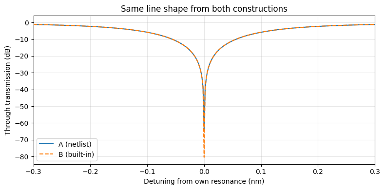
# overlay both line shapes on a common detuning axis
plt.figure(figsize=(8, 4))
for (name, r), style in [(("A (netlist)", res_a), "-"), (("B (built-in)", res_b), "--")]:
plt.plot(
(r["wl"] - r["lam_res"]) * 1e3, 10 * np.log10(r["trans"]), style, label=name
)
plt.xlabel("Detuning from own resonance (nm)")
plt.ylabel("Through transmission (dB)")
plt.title("Same line shape from both constructions")
plt.xlim(-0.3, 0.3)
plt.legend()
plt.grid(True, alpha=0.3)
plt.tight_layout()
plt.show()
A (netlist): resonance 1552.627 nm   Q 4600   FWHM 42.0 GHz
B (built-in): resonance 1550.346 nm   Q 4619   FWHM 41.9 GHz
photon-lifetime bandwidth: 21.0 GHz
Coupled-mode reference
Müller et al. derive the small-signal EO response from perturbation of the intracavity field. In the lossless-detuning limit (their Eq. 3) it is a sum of two sideband terms,
with cavity field lifetime \(\tau_a\) and detuning \(\Delta=\omega_r-\omega_0\). When \(\omega_m\approx|\Delta|\) the first term collapses to \(1/\tau_a\) and the response peaks; at zero detuning it reduces to a single-pole low-pass at \(1/(2\pi\tau_a)\).
[5]:
def cmt_s21(f_m, detuning_hz, tau_a):
    """Closed-form small-signal EO response (Mueller et al., Eq. 3, symmetric form)."""
    wm = 2 * np.pi * np.asarray(f_m)
    g = 1.0 / tau_a  # cavity field decay rate
    det = 2 * np.pi * detuning_hz
    # two sideband terms; the first one peaks when wm ~ |det|
    return 1.0 / (g + 1j * (wm - det)) + 1.0 / (g + 1j * (wm + det))
Time-domain link and impulse-response extraction
The full link - CW laser → ring → photodiode - is one parametric component taking the laser detuning and the ring construction. The stepper runs in a frame at the carrier f_laser, and both PhaseModTimeStepper and RingTimeStepper re-reference the modulator index to that carrier internally from reference_frequency, so no manual index updates are needed. (The ring mode number is ~170, so the resonance is hypersensitive to n_eff - a \(10^{-4}\) shift moves it several
GHz - which is exactly why this correction matters.)
We read the EO response from an optical monitor on the port feeding the photodiode (FFT of the optical power), not the detector output - the realistic photodiode model (responsivity, saturation, noise, 65 GHz bandwidth) therefore has no effect on the measurement.
The three source/sink components are created with the pfa abstract API:
pfa.cw_laser(power=...)- CW optical pump that injects a constant-amplitude field into optical portP0.pfa.signal_source(..., waveform="gaussian")- electrical pulse generator;amplitudeis in \(\text{V}/\sqrt{\Omega}\),widthandstartare expressed as fractions of the sourceperiod. Connected to the ring’s drive port via electrical portE0.pfa.photodiode(...)- realistic detector (responsivity, gain, saturation, noise, Butterworth roll-off); exposes optical portP0and electrical portE0directly (noadd_portneeded).
The small Gaussian electrical pulse produced by pfa.signal_source is wired directly to the modulator’s drive port; the actual drive is read back from an electrical monitor on the same port and used as the FFT denominator. dt is fixed (~0.025 ps, ~35 steps per round trip).
[6]:
dt = 0.025e-12  # time step (s), ~35 steps per cavity round trip
settle = 8000  # transient steps before measurement (cavity fill-up)
# fixed pole-residue fit window for the optical models (independent of f_m)
freq_window = np.linspace(freq0 - 300e9, freq0 + 300e9, 120)

# gaussian drive pulse: short -> excites the whole band of interest at once
sigma = 0.8e-12  # pulse width (s)
v_peak = 0.01  # pulse amplitude (V); kept small for small-signal linearity
t_imp = (settle + 1000) * dt  # pulse center, shortly after the transient
pulse_period = 2e-9  # source period > record length -> exactly one pulse fires


def ring_port_names(use_builtin):
    """(input, through, drive) port names for the chosen ring construction."""
    return ("P0", "P1", "E0") if use_builtin else ("In", "Through", "E_drive")


@pf.parametric_component
def create_link(detuning_hz=0.0, use_builtin=False):
    """CW laser -> dispersion-compensated ring (either construction) -> photodiode."""
    res = res_b if use_builtin else res_a  # each ring uses its own resonance
    f_laser = res["f_res"] - detuning_hz
    # the steppers re-reference the ring index to the laser carrier internally
    create = create_ring_builtin if use_builtin else create_ring_netlist
    ring = create()
    in_p, thru_p, drv_p = ring_port_names(use_builtin)

    # CW pump laser (1 mW)
    laser = pfa.cw_laser(power=1e-3)

    # gaussian pulse generator driving the modulator port
    fwhm = 2 * np.sqrt(2 * np.log(2)) * sigma
    drv = pfa.signal_source(
        frequency=1 / pulse_period,
        amplitude=v_peak / np.sqrt(z0),
        waveform="gaussian",
        width=fwhm / pulse_period,
        start=t_imp - np.sqrt(2 * np.log(1e3)) * sigma,
    )

    pd = pfa.photodiode(
        responsivity=0.85,
        gain=50.0,
        saturation_current=6.8e-3,
        dark_current=10e-9,
        thermal_noise=3.3e-22,
        filter_frequency=65e9,
        roll_off=2,
    )

    # wire the link: laser -> ring -> PD, pulse generator -> ring drive
    return pf.component_from_netlist(
        {
            "name": "MRM_link",
            "instances": {
                # rotate the laser 180 deg so its source port faces the ring input
                # in this virtual-port circuit (pfa.cw_laser emits along its port axis)
                "laser": {"component": laser, "rotation": 180},
                "ring": {"component": ring},
                "pd": {"component": pd},
                "drv": {"component": drv},
            },
            "virtual connections": [
                (("laser", "P0"), ("ring", in_p)),
                (("pd", "P0"), ("ring", thru_p)),
                (("drv", "E0"), ("ring", drv_p)),
            ],
            "ports": [("pd", "E0", "rx")],
            "models": [(pf.CircuitModel(), "Circuit")],
        }
    )


link = create_link()  # built once; retuned per run with link.update(...)


def impulse_response(detuning_hz, use_builtin=False, record=32000):
    """EO response over the whole band from one electrical pulse: H(f)=FFT(dP)/FFT(dV)."""
    link.update(detuning_hz=detuning_hz, use_builtin=use_builtin)
    res = res_b if use_builtin else res_a
    f_laser = res["f_res"] - detuning_hz
    _, thru_p, drv_p = ring_port_names(use_builtin)
    ring_ref = next(
        r
        for r in link.references
        if r.component.name.startswith(("AllPassMRM", "Ring Resonator"))
    )
    n = settle + record
    # monitors: optical power feeding the PD + electrical pulse at the modulator
    ts = link.setup_time_stepper(
        time_step=dt,
        carrier_frequency=f_laser,
        time_stepper_kwargs={
            "frequencies": freq_window,
            "monitors": {"opt_in": ring_ref[thru_p], "v_drive": ring_ref[drv_p]},
        },
    )
    ts.reset()
    out = ts.step(steps=n, time_step=dt)  # no external input: PulseGen is the drive
    power = np.abs(np.asarray(out["opt_in@0+"])) ** 2  # optical power before the PD
    volts = np.real(np.asarray(out["v_drive@0-"])) * np.sqrt(z0)  # pulse into the ring
    base = np.mean(power[settle - 2000 : settle - 400])  # clean pre-pulse baseline
    w = slice(settle - 400, n)  # analysis window: just before the pulse to the end
    d_power = power[w] - base  # power perturbation = impulse response
    d_volts = volts[w]
    freqs = np.fft.rfftfreq(d_power.size, dt)
    v_spec = np.fft.rfft(d_volts)
    mask = (
        np.abs(v_spec) > 0.05 * np.abs(v_spec).max()
    )  # trust only the well-excited band
    h = np.fft.rfft(d_power)[mask] / v_spec[mask]  # transfer function dP/dV
    return freqs[mask], h
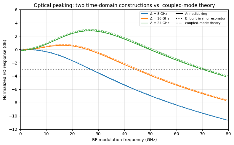
Optical peaking vs. detuning - both approaches against CMT
For each detuning, one impulse-response simulation per construction: Approach A (solid), Approach B (dotted), and the CMT model (dashed, using \(\tau_a\) from Approach A - the two values agree to <0.5%). All curves are normalized at 4 GHz.
[7]:
detunings_ghz = [8.0, 16.0, 24.0]  # laser-resonance detunings to compare
f_fine = np.linspace(1e9, 80e9, 400)  # frequency grid for the CMT curves
colors = ["C0", "C1", "C2"]


def to_db(x, ref):
    return 20 * np.log10(np.abs(x) / np.abs(ref))


fig, ax = plt.subplots(figsize=(8, 5))
for det_ghz, col in zip(detunings_ghz, colors):
    det = det_ghz * 1e9
    curves = {}
    for use_builtin in (False, True):  # one simulation per construction
        f_imp, h_imp = impulse_response(det, use_builtin=use_builtin)
        keep = f_imp <= 80e9
        ref_imp = h_imp[np.argmin(np.abs(f_imp - 4e9))]  # normalize at low frequency
        curves[use_builtin] = (f_imp[keep], to_db(h_imp[keep], ref_imp))
    ax.plot(curves[False][0] / 1e9, curves[False][1], "-", color=col,
            label=f"Δ = {det_ghz:.0f} GHz")
    ax.plot(curves[True][0] / 1e9, curves[True][1], ":", color=col, lw=2.2)
    # analytic CMT reference, normalized the same way (dashed)
    h_cmt = cmt_s21(f_fine, det, res_a["tau_a"])
    ax.plot(f_fine / 1e9, to_db(h_cmt, cmt_s21(1e6, det, res_a["tau_a"])),
            "--", color=col, alpha=0.6)
    # quantify approach A vs B agreement on a common grid
    diff = np.abs(
        curves[False][1]
        - np.interp(curves[False][0], curves[True][0], curves[True][1])
    )
    print(f"Δ = {det_ghz:>4.0f} GHz: max |A - B| = {diff.max():.3f} dB")

ax.axhline(-3, color="gray", ls=":")
ax.plot([], [], "k-", label="A: netlist ring")
ax.plot([], [], "k:", lw=2.2, label="B: built-in ring resonator")
ax.plot([], [], "k--", alpha=0.6, label="coupled-mode theory")
ax.set_xlabel("RF modulation frequency (GHz)")
ax.set_ylabel("Normalized EO response (dB)")
ax.set_title("Optical peaking: two time-domain constructions vs. coupled-mode theory")
ax.legend(ncol=2, fontsize=8)
ax.grid(True, alpha=0.3)
ax.set_ylim(-12, 6)
ax.set_xlim(0, 80)
fig.tight_layout()
plt.show()

print(f"photon-lifetime bandwidth (Δ=0): {photon_bw/1e9:.1f} GHz")
Δ =    8 GHz: max |A - B| = 0.065 dB
Δ =   16 GHz: max |A - B| = 0.063 dB
Δ =   24 GHz: max |A - B| = 0.063 dB
photon-lifetime bandwidth (Δ=0): 21.0 GHz
Summary
Both constructions reproduce optical peaking and match the CMT model through 70 GHz: a clean low-pass at small detuning and a peak near \(f_m\approx|\Delta|\) that extends the bandwidth past the photon-lifetime limit \(1/(2\pi\tau_a)\). The two PhotonForge results also agree with each other to a few hundredths of a dB - they are numerically equivalent descriptions of the same cavity.
Approach A (netlist) solves the cavity as explicit circuit feedback (coupler + active waveguide +
CircuitTimeStepper): more verbose, but it generalizes to arbitrary intra-cavity topologies (separate active/passive sections, multiple couplers, embedded filters).Approach B (built-in) packs the same physics into a single
RingModel/RingTimeSteppercomponent (bus coupler + round-trip delay line, modulation viadn_dv\(=\lambda_0/(2V_\pi L)\)): far more compact when the standard single- or double-bus ring is all you need.The built-in coupler convention (\(\tau = -i\,e^{i\arg\kappa}\sqrt{1-|\kappa|^2}\)) shifts the resonance comb by a quarter FSR relative to the netlist coupler - harmless, since each ring is characterized around its own resonance and driven at the same detunings.
The peaking is produced entirely by the cavity dynamics solved in the time domain: no electrical reactance exists anywhere in either circuit (
f_3dB=0).