Mach-Zehnder Modulator

The Mach-Zehnder modulator (MZM) is the workhorse intensity modulator of optical communications. The MZMTimeStepper provides it as a single, ready-made time-domain model, so a transmitter can be assembled without building the interferometer out of couplers and phase shifters. The model simulates the interference of the two arms,

\[A_\mathrm{out} = A_\mathrm{in} \left( w_1 e^{j \phi_1} + w_2 e^{-j \phi_2} \right) \qquad \phi_{1,2} = \frac{\pi V_{1,2}}{V_\pi} + k_2 V_{1,2}^2 + k_3 V_{1,2}^3\]

where the arm weights \(w_1\) and \(w_2\) account for the insertion loss and extinction ratio, and a constant phase_bias (in degrees) is added to \(\phi_1\) to set the operating point. In the default push-pull configuration a single electrical port drives both arms in opposition (\(V_2 = V_1\)); the dual-drive configuration exposes two independent electrical ports. A first-order low-pass filter (f_3dB) models the finite electrical bandwidth.

This guide covers the static transfer function and its non-idealities, digital modulation at the quadrature point with bandwidth-limited eye diagrams, and the difference between push-pull, single-arm, and phase-only operation with dual drive.

Setup

import matplotlib.pyplot as plt
import numpy as np
import photonforge as pf
import photonforge.abstract as pfa

viewer = pf.live_viewer.LiveViewer()

LiveViewer started at http://localhost:49172

tech = pf.basic_technology()
pf.config.default_technology = tech

lda0 = 1.55
f0 = pf.C_0 / lda0
z0 = 50.0
v_pi = 4.0
time_step = 1e-12

Static Transfer Function

The abstract mach_zehnder_modulator component has two optical ports and, in push-pull mode, a single electrical drive E0. We use \(V_\pi = 4\) V, representative of silicon depletion-mode devices.

modulator = pfa.mach_zehnder_modulator(v_pi=v_pi)
viewer(modulator)

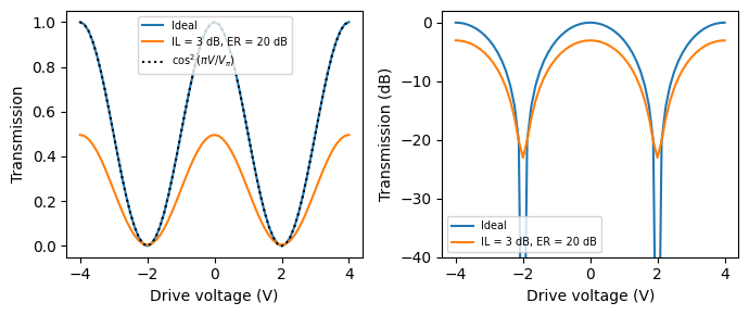
Sweeping a DC voltage from a signal_source traces the interferometric transfer function. In push-pull operation both arms move in opposite directions, so the accumulated phase difference is \(2 \pi V / V_\pi\) and the power transmission is

\[T(V) = \cos^2 \left( \frac{\pi V}{V_\pi} \right)\]

reaching the first null at \(V_\pi / 2\). Alongside the ideal device we sweep one with 3 dB insertion loss and a 20 dB extinction ratio: the insertion loss lowers the transmission maxima, while the finite extinction ratio, caused by imbalanced arm losses in a real device, limits how deep the nulls go.

devices = {
    "Ideal": pfa.mach_zehnder_modulator(v_pi=v_pi),
    "IL = 3 dB, ER = 20 dB": pfa.mach_zehnder_modulator(
        v_pi=v_pi, insertion_loss=3, extinction_ratio=20
    ),
}

bias_voltages = np.linspace(-4, 4, 65)
num_steps = 100

fig, (ax1, ax2) = plt.subplots(1, 2, figsize=(7, 3), tight_layout=True)
for label, device in devices.items():
    source = pfa.signal_source(amplitude=0, offset=0)
    link = pf.Component("dc_link")
    laser_ref = link.add_reference(pfa.cw_laser(power=1e-3))
    modulator_ref = link.add_reference(device)
    source_ref = link.add_reference(source)
    modulator_ref.connect("P0", laser_ref["P0"])
    source_ref.connect("E0", modulator_ref["E0"])
    link.add_port(modulator_ref["P1"], "out")
    link.add_model(pf.CircuitModel(), "Circuit")

    transmission = []
    for voltage in bias_voltages:
        source.update(offset=voltage / np.sqrt(z0))
        time_stepper = link.setup_time_stepper(
            time_step=time_step, carrier_frequency=f0, show_progress=False
        )
        a = time_stepper.step(steps=num_steps, time_step=time_step, show_progress=False)["out@0"]
        transmission.append(np.abs(a[-1]) ** 2 / 1e-3)
    transmission = np.array(transmission)
    ax1.plot(bias_voltages, transmission, label=label)
    ax2.plot(bias_voltages, 10 * np.log10(np.maximum(transmission, 1e-8)), label=label)

ax1.plot(bias_voltages, np.cos(np.pi * bias_voltages / v_pi) ** 2, "k:", label="$\\cos^2(\\pi V / V_\\pi)$")
ax1.set(xlabel="Drive voltage (V)", ylabel="Transmission")
ax2.set(xlabel="Drive voltage (V)", ylabel="Transmission (dB)", ylim=(-40, 2))
ax1.legend(fontsize=7)
_ = ax2.legend(fontsize=7)

Digital Modulation at Quadrature

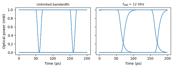
Setting phase_bias to 90° places the zero-volt operating point at quadrature, the center of the linear region, so a bipolar drive between \(-V_\pi / 4\) and \(+V_\pi / 4\) swings the output over its full range. We drive the modulator with a 10 Gb/s NRZ PRBS7 pattern and fold the optical output power into an eye diagram.

The f_3dB argument shows its effect here: with the electrical bandwidth limited to 12 GHz, close to the bit rate, the edges slow down and intersymbol interference starts to close the eye.

This is a lumped modulator model: the interferometer responds instantaneously to the filtered drive voltage, and f_3dB stands in for the aggregate electrical bandwidth of the driver, electrodes, and junction. The traveling-wave nature of high-speed electrodes, where the RF drive co-propagates with the light and the bandwidth is set by velocity matching, RF loss, and termination, is not captured at this level of abstraction. When those effects matter, model each arm with the traveling-wave TerminatedModTimeStepper phase modulator and assemble the interferometer explicitly from couplers.

bit_rate = 10e9
time_step_eye = 0.25e-12
unit_interval = int(round(1 / bit_rate / time_step_eye))
num_bits = 256
t_eye = np.arange(2 * unit_interval) * time_step_eye

cases = {
    "Unlimited bandwidth": 0,
    "$f_{3\\mathrm{dB}}$ = 12 GHz": 12e9,
}

fig, axes = plt.subplots(1, 2, figsize=(7, 2.8), sharey=True, tight_layout=True)
for ax, (label, f_3db) in zip(axes, cases.items()):
    modulator_tx = pfa.mach_zehnder_modulator(v_pi=v_pi, phase_bias=90, f_3dB=f_3db)
    source = pfa.signal_source(
        frequency=bit_rate,
        amplitude=(v_pi / 2) / np.sqrt(z0),
        offset=(-v_pi / 4) / np.sqrt(z0),
        waveform="trapezoid",
        rise=0.1,
        fall=0.1,
        width=1.1,
        prbs=7,
        seed=0,
    )
    transmitter = pf.Component("transmitter")
    laser_ref = transmitter.add_reference(pfa.cw_laser(power=1e-3))
    modulator_ref = transmitter.add_reference(modulator_tx)
    source_ref = transmitter.add_reference(source)
    modulator_ref.connect("P0", laser_ref["P0"])
    source_ref.connect("E0", modulator_ref["E0"])
    transmitter.add_port(modulator_ref["P1"], "out")
    transmitter.add_model(pf.CircuitModel(), "Circuit")

    num_steps = unit_interval * num_bits
    time_stepper = transmitter.setup_time_stepper(
        time_step=time_step_eye, carrier_frequency=f0, show_progress=False
    )
    output = time_stepper.step(steps=num_steps, time_step=time_step_eye, show_progress=False)
    power = np.abs(output["out@0"]) ** 2

    segments = power[unit_interval // 2 :]
    segments = segments[: len(segments) // (2 * unit_interval) * 2 * unit_interval]
    for segment in segments.reshape(-1, 2 * unit_interval):
        ax.plot(t_eye * 1e12, segment * 1e3, color="C0", alpha=0.15, linewidth=0.8)
    ax.set_title(label, fontsize=9)
    ax.set_xlabel("Time (ps)")
axes[0].set_ylabel("Optical power (mW)")
plt.show()

Dual Drive and Chirp

With drive="dual" the two arms are driven independently through E0 and E1, which controls not only the output power but also its phase, the chirp of the modulated signal. Three static drive schemes illustrate the range of behaviors:

• Opposing drives (\(V_2 = V_1\), reproducing push-pull): the common phase cancels and the output is a chirp-free intensity modulation.

• Equal drives (\(V_2 = -V_1\), moving both arms together): the interference never changes, and the device becomes a pure phase modulator with constant output power.

• Single-arm drive (\(V_2 = 0\)): the modulation depth is halved and the output carries a residual phase modulation, the chirp typical of single-drive modulators.

One practical detail: parametric components with identical arguments refer to the same shared component, so the two drive sources must be created with some distinguishing argument (here, different seed values) to remain independent.

modulator_dual = pfa.mach_zehnder_modulator(drive="dual", v_pi=v_pi)
source_1 = pfa.signal_source(amplitude=0, offset=0, seed=1)
source_2 = pfa.signal_source(amplitude=0, offset=0, seed=2)

dual_link = pf.Component("dual_link")
laser_ref = dual_link.add_reference(pfa.cw_laser(power=1e-3))
modulator_ref = dual_link.add_reference(modulator_dual)
source_1_ref = dual_link.add_reference(source_1)
source_2_ref = dual_link.add_reference(source_2)
modulator_ref.connect("P0", laser_ref["P0"])
source_1_ref.connect("E0", modulator_ref["E0"])
source_2_ref.connect("E0", modulator_ref["E1"])
dual_link.add_port(modulator_ref["P1"], "out")
dual_link.add_model(pf.CircuitModel(), "Circuit")

schemes = {
    "Opposing, $V_2 = V_1$": 1.0,
    "Equal, $V_2 = -V_1$": -1.0,
    "Single arm, $V_2 = 0$": 0.0,
}

voltages = np.linspace(-1.8, 1.8, 31)
fig, (ax1, ax2) = plt.subplots(1, 2, figsize=(7, 3), tight_layout=True)
for label, ratio in schemes.items():
    transmission = []
    phase = []
    for voltage in voltages:
        source_1.update(offset=voltage / np.sqrt(z0))
        source_2.update(offset=ratio * voltage / np.sqrt(z0))
        time_stepper = dual_link.setup_time_stepper(
            time_step=time_step, carrier_frequency=f0, show_progress=False
        )
        a = time_stepper.step(steps=100, time_step=time_step, show_progress=False)["out@0"]
        transmission.append(np.abs(a[-1]) ** 2 / 1e-3)
        phase.append(np.angle(a[-1]))
    ax1.plot(voltages, transmission, label=label)
    ax2.plot(voltages, np.unwrap(np.array(phase)), label=label)

ax1.set(xlabel="$V_1$ (V)", ylabel="Transmission")
ax2.set(xlabel="$V_1$ (V)", ylabel="Output phase (rad)")
ax1.legend(fontsize=7)
_ = ax2.legend(fontsize=7)

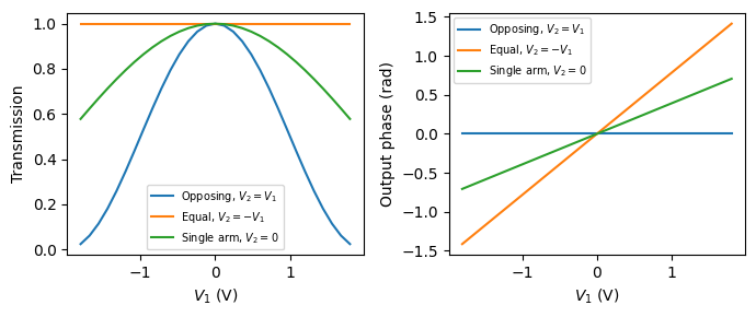
Note that the sign convention of the second arm follows the model equation: because \(\phi_2\) enters as \(e^{-j \phi_2}\), driving both electrical ports with the same voltage produces the opposing, push-pull behavior, while \(V_2 = -V_1\) moves the arms together.

Summary

• pfa.mach_zehnder_modulator is a complete MZM in a single component: push-pull by default (E0 only) or dual-drive (E0, E1) with drive="dual".

• In push-pull operation the transmission is \(\cos^2(\pi V / V_\pi)\), with the first null at \(V_\pi / 2\); phase_bias (in degrees) sets the static operating point, with 90° placing zero volts at quadrature.

• insertion_loss lowers the transmission maxima and extinction_ratio limits the depth of the nulls; f_3dB models the electrical bandwidth and its intersymbol interference.

• Dual drive controls chirp: same-voltage drives give chirp-free intensity modulation, opposite voltages give pure phase modulation, and single-arm drive gives chirped modulation at half depth.

• The same nonlinear phase (\(k_2\), \(k_3\)) and voltage-dependent loss terms as the PhaseModTimeStepper are available, and when arm-level or traveling-wave electrode detail matters, the interferometer can be assembled explicitly from lumped or traveling-wave phase modulators and couplers.

• Parametric components with identical arguments are shared objects; give independent sources a distinguishing argument.