Traveling-Wave Modulator

At high speeds, a modulator electrode can no longer be treated as a single lumped node: it becomes a transmission line, and the drive signal travels along it together with the light. The TerminatedModTimeStepper models this traveling-wave electro-optic phase modulator. The RF wave is launched at one end of the electrode, co-propagates with the optical mode over the modulator length, and is absorbed by the load impedance at the far end, which is why the model has a single electrical port and takes its name from the terminated line.

The optical phase accumulates from the local voltage seen along the propagation, so the response depends on how well the RF wave keeps up with the light. Three ingredients set the modulation bandwidth: the velocity mismatch between the RF index \(n_\mathrm{RF}\) and the optical group index \(n_g\), the RF propagation loss, and reflections from imperfect source and load impedances. This is in contrast with the lumped PhaseModTimeStepper, covered in the Phase Modulator guide, where the bandwidth is a simple first-order filter.

The electrical input amplitude is converted to the launched voltage as \(V = \Re \lbrace A \rbrace \sqrt{Z_\mathrm{source}}\). This guide covers the static phase law, the frequency response under velocity mismatch and RF loss, and the effect of termination mismatch.

Setup

import matplotlib.pyplot as plt
import numpy as np
import photonforge as pf
import photonforge.abstract as pfa

viewer = pf.live_viewer.LiveViewer()

LiveViewer started at http://localhost:54950

tech = pf.basic_technology()
pf.config.default_technology = tech

lda0 = 1.55
f0 = pf.C_0 / lda0
z0 = 50.0
time_step = 0.1e-12

The Modulator and Its Static Response

The abstract terminated_modulator has two optical ports and the single electrical port of the terminated line. We use a 3 mm long device with \(V_{\pi L} = 2\) V·cm, so \(V_\pi = V_{\pi L} / \ell \approx 6.7\) V, an optical group index \(n_g = 4.2\), and, for now, a perfectly velocity-matched RF index \(n_\mathrm{RF} = n_g\) with matched source and load impedances (the defaults). When the model is attached to a real layout component instead of the abstract symbol, n_eff, n_group, n_rf, and z0 can also be computed automatically by mode-solving the port cross sections.

length = 3000.0
v_pil = 20000.0
v_pi = v_pil / length
n_group = 4.2

modulator = pfa.terminated_modulator(length=length, v_piL=v_pil)
viewer(modulator)

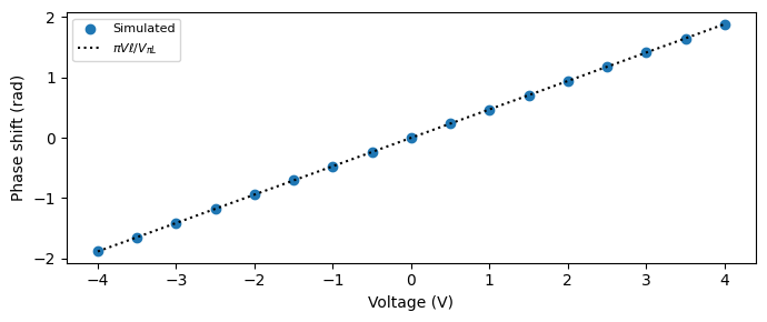
At DC, the whole line settles to the drive voltage and the accumulated phase follows the same law as the lumped phase modulator, \(\Delta \phi = \pi V \ell / V_{\pi L}\), plotted below with the analytic line as a dotted reference. The nonlinear \(k_2\) and \(k_3\) terms are also available and behave as in the lumped model.

source = pfa.signal_source(amplitude=0, offset=0)
link = pf.Component("dc_link")
laser_ref = link.add_reference(pfa.cw_laser(power=1e-3))
modulator_ref = link.add_reference(modulator)
source_ref = link.add_reference(source)
modulator_ref.connect("P0", laser_ref["P0"])
source_ref.connect("E0", modulator_ref["E0"])
link.add_port(modulator_ref["P1"], "out")
link.add_model(pf.CircuitModel(), "Circuit")

voltages = np.linspace(-4, 4, 17)
phases = []
for voltage in voltages:
    source.update(offset=voltage / np.sqrt(z0))
    time_stepper = link.setup_time_stepper(
        time_step=time_step, carrier_frequency=f0, show_progress=False
    )
    a = time_stepper.step(steps=2000, time_step=time_step, show_progress=False)["out@0"]
    phases.append(np.angle(a[-1]))
phases = np.unwrap(np.array(phases))

fig, ax = plt.subplots(figsize=(7, 3), tight_layout=True)
ax.plot(voltages, phases - phases[len(voltages) // 2], "o", label="Simulated")
ax.plot(voltages, np.pi * voltages / v_pi, "k:", label="$\\pi V \\ell / V_{\\pi L}$")
ax.set(xlabel="Voltage (V)", ylabel="Phase shift (rad)")
_ = ax.legend(fontsize=8)

Frequency Response: Velocity Matching, Walk-Off, and RF Loss

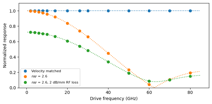
As the drive frequency increases, the RF wave and the optical pulse must stay in step over the full electrode length. The optical envelope travels at the group velocity \(c_0 / n_g\) while the RF wave travels at \(c_0 / n_\mathrm{RF}\); a mismatch makes the light slide past the RF wave, averaging out the modulation.

The model implements the full transmission-line dynamics. With the RF propagation constant \(\gamma = \alpha_\mathrm{RF} + j 2 \pi f n_\mathrm{RF} / c_0\), the optical phase constant \(\beta_o = 2 \pi f n_g / c_0\), and the line input impedance \(Z_\mathrm{in} = Z_0 (Z_l + Z_0 \tanh \gamma \ell) / (Z_0 + Z_l \tanh \gamma \ell)\), the electro-optic transfer function is

\[H(f) = \frac{-2 Z_\mathrm{in}}{Z_\mathrm{in} + Z_s} \, \frac{(Z_l + Z_0) F_+ + (Z_l - Z_0) F_-}{(Z_l + Z_0) e^{\gamma \ell} + (Z_l - Z_0) e^{-\gamma \ell}} \qquad F_\pm = \frac{1 - e^{(\pm \gamma - j \beta_o) \ell}}{(\pm \gamma - j \beta_o) \ell}\]

normalized so that an ideal device gives \(\lvert H \rvert = 1\) at DC. The terms \(F_+\) and \(F_-\) are the overlap integrals of the light with the forward-traveling RF wave and with the wave reflected from the load. For matched terminations (\(Z_l = Z_s = Z_0\)) only the forward wave survives and the magnitude reduces to

\[\lvert H(f) \rvert = \left\lvert \frac{1 - e^{-g}}{g} \right\rvert \qquad g = \left( \alpha_\mathrm{RF} + j \frac{2 \pi f (n_\mathrm{RF} - n_g)}{c_0} \right) \ell\]

the walk-off response, which becomes \(\mathrm{sinc}(\pi f (n_\mathrm{RF} - n_g) \ell / c_0)\) without RF loss, with a null when the walk-off equals one RF period.

We sweep the drive frequency and extract the modulation index from the output envelope phase for three devices: velocity-matched, mismatched with \(n_\mathrm{RF} = 2.6\) (an unloaded coplanar electrode on silicon, against \(n_g = 4.2\)), and the same mismatched line with 2 dB/mm of RF loss. The transfer function above is drawn as dotted lines for reference. Velocity matching is what keeps the response flat far beyond the walk-off limit, and RF loss both lowers the overall efficiency and softens the walk-off nulls.

drive_freqs = np.array(
    [2e9, 4e9, 6e9, 8e9, 10e9, 14e9, 20e9, 26e9, 30e9, 40e9, 50e9, 60e9, 70e9, 80e9]
)
freq_fine = np.linspace(0.5e9, 85e9, 400)
v_small = 0.2
m_dc = np.pi * v_small / v_pi

devices = {
    "Velocity matched": {"n_rf": n_group},
    "$n_{RF}$ = 2.6": {"n_rf": 2.6},
    "$n_{RF}$ = 2.6, 2 dB/mm RF loss": {"n_rf": 2.6, "rf_propagation_loss": 2e-3},
}

def eo_s21(freqs, n_rf, rf_loss=0.0, z_load=z0, z_source=z0):
    omega = 2 * np.pi * freqs
    alpha = rf_loss / (20 * np.log10(np.e)) + 1e-15
    gl = (alpha + 1j * omega / pf.C_0 * n_rf) * length
    tgl = np.tanh(gl)
    z_in = z0 * (z_load + z0 * tgl) / (z0 + z_load * tgl)
    jf = 1j * omega / pf.C_0 * n_group * length
    f_p = (1 - np.exp(gl - jf)) / (gl - jf)
    f_m = (1 - np.exp(-gl - jf)) / (-gl - jf)
    return (-2 * z_in / (z_in + z_source) * ((z_load + z0) * f_p + (z_load - z0) * f_m)) / (
        (z_load + z0) * np.exp(gl) + (z_load - z0) * np.exp(-gl)
    )

num_steps = 10000
t = np.arange(num_steps) * time_step
settled = slice(num_steps // 2, None)

fig, ax = plt.subplots(figsize=(7, 3.5), tight_layout=True)
for i, (label, kwargs) in enumerate(devices.items()):
    modulator_bw = pfa.terminated_modulator(length=length, v_piL=v_pil, **kwargs)
    source_bw = pfa.signal_source(frequency=10e9, amplitude=v_small / np.sqrt(z0))
    link_bw = pf.Component(f"bw_link_{i}")
    laser_ref = link_bw.add_reference(pfa.cw_laser(power=1e-3))
    modulator_ref = link_bw.add_reference(modulator_bw)
    source_ref = link_bw.add_reference(source_bw)
    modulator_ref.connect("P0", laser_ref["P0"])
    source_ref.connect("E0", modulator_ref["E0"])
    link_bw.add_port(modulator_ref["P1"], "out")
    link_bw.add_model(pf.CircuitModel(), "Circuit")

    measured = []
    for drive_freq in drive_freqs:
        source_bw.update(frequency=drive_freq)
        time_stepper = link_bw.setup_time_stepper(
            time_step=time_step, carrier_frequency=f0, show_progress=False
        )
        a = time_stepper.step(steps=num_steps, time_step=time_step, show_progress=False)["out@0"]
        phase = np.unwrap(np.angle(a))[settled]
        tone = 2 * np.abs(
            np.mean((phase - phase.mean()) * np.exp(-2j * np.pi * drive_freq * t[settled]))
        )
        measured.append(tone / m_dc)
    ax.plot(drive_freqs / 1e9, measured, "o", color=f"C{i}", label=label)
    ax.plot(
        freq_fine / 1e9,
        np.abs(eo_s21(freq_fine, kwargs["n_rf"], kwargs.get("rf_propagation_loss", 0.0))),
        ":",
        color=f"C{i}",
    )

ax.set(xlabel="Drive frequency (GHz)", ylabel="Normalized response", ylim=(0, 1.1))
_ = ax.legend(fontsize=8)

Termination Mismatch

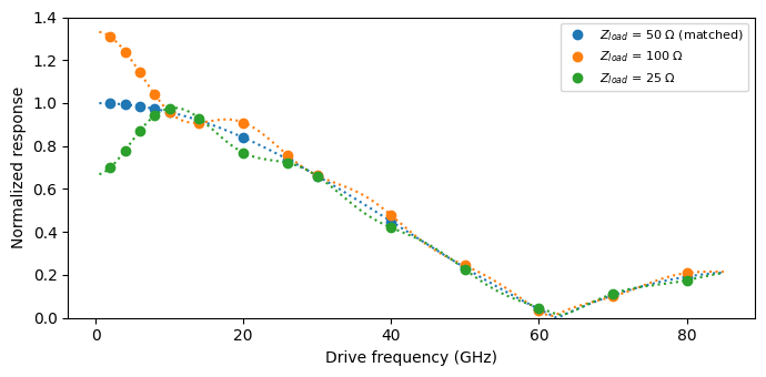
The far end of the electrode is closed by z_load (and the source side by z_source, both matched to the line impedance by default). When the load does not match the line, part of the RF wave reflects with coefficient \(\Gamma = (Z_l - Z_0) / (Z_l + Z_0)\) and travels backward against the light, entering the transfer function through the \(F_-\) term and the input impedance. At low frequency the standing voltage scales the response by \(1 + \Gamma\), while at higher frequencies the counter-propagating wave walks off very quickly and mostly adds ripple.

We compare the matched termination with a 100 Ω load (\(\Gamma = +1/3\)) and a 25 Ω load (\(\Gamma = -1/3\)), keeping the mismatched RF index from the previous section. The dotted lines show the same transfer function evaluated with each load.

loads = {
    "$Z_{load}$ = 50 Ω (matched)": 50.0,
    "$Z_{load}$ = 100 Ω": 100.0,
    "$Z_{load}$ = 25 Ω": 25.0,
}

fig, ax = plt.subplots(figsize=(7, 3.5), tight_layout=True)
for i, (label, z_load) in enumerate(loads.items()):
    modulator_term = pfa.terminated_modulator(
        length=length, v_piL=v_pil, n_rf=2.6, z_load=z_load
    )
    source_term = pfa.signal_source(frequency=10e9, amplitude=v_small / np.sqrt(z0))
    link_term = pf.Component(f"term_link_{i}")
    laser_ref = link_term.add_reference(pfa.cw_laser(power=1e-3))
    modulator_ref = link_term.add_reference(modulator_term)
    source_ref = link_term.add_reference(source_term)
    modulator_ref.connect("P0", laser_ref["P0"])
    source_ref.connect("E0", modulator_ref["E0"])
    link_term.add_port(modulator_ref["P1"], "out")
    link_term.add_model(pf.CircuitModel(), "Circuit")

    measured = []
    for drive_freq in drive_freqs:
        source_term.update(frequency=drive_freq)
        time_stepper = link_term.setup_time_stepper(
            time_step=time_step, carrier_frequency=f0, show_progress=False
        )
        a = time_stepper.step(steps=num_steps, time_step=time_step, show_progress=False)["out@0"]
        phase = np.unwrap(np.angle(a))[settled]
        tone = 2 * np.abs(
            np.mean((phase - phase.mean()) * np.exp(-2j * np.pi * drive_freq * t[settled]))
        )
        measured.append(tone / m_dc)
    ax.plot(drive_freqs / 1e9, measured, "o", color=f"C{i}", label=label)
    ax.plot(freq_fine / 1e9, np.abs(eo_s21(freq_fine, 2.6, z_load=z_load)), ":", color=f"C{i}")

ax.set(xlabel="Drive frequency (GHz)", ylabel="Normalized response", ylim=(0, 1.4))
_ = ax.legend(fontsize=8)

Summary

• pfa.terminated_modulator models a traveling-wave phase modulator with a terminated electrode: one electrical port, with the launched voltage \(V = \Re \lbrace A \rbrace \sqrt{Z_\mathrm{source}}\).

• At DC the phase follows \(\pi V \ell / V_{\pi L}\), with the same nonlinear \(k_2\), \(k_3\) terms and optical propagation loss as the lumped phase modulator.

• The bandwidth is set by physics rather than a filter: velocity mismatch between \(n_\mathrm{RF}\) and the optical group index produces the walk-off sinc response, and rf_propagation_loss lowers the efficiency and softens the nulls.

• z_load and z_source control the line terminations; a mismatched load reflects the RF wave, scaling the low-frequency response by \(1 + \Gamma\) and adding ripple.

• With n_eff, n_group, n_rf, or z0 left as None on a layout component, the model extracts them by mode-solving the port cross sections, connecting the time-domain response directly to the physical design.

• For the lumped counterpart with a first-order electrical bandwidth, see the Phase Modulator guide.