CW Laser

Time-domain circuit simulations in PhotonForge are built on time steppers: time-domain models that advance the signals in a photonic circuit sample by sample. Instead of the full optical field, time steppers operate on the slowly varying complex envelope around a global carrier frequency, and optical amplitudes are expressed in units of \(\sqrt{\mathrm{W}}\), so \(\lvert a \rvert^2\) is the instantaneous optical power.

Every time-domain simulation starts with a source. The CWLaserTimeStepper models a continuous-wave (CW) laser that emits the complex field

\[a[k] = \sqrt{P[k]} \, e^{j \phi[k]}\]

By default the source is ideal, with constant power and constant phase. Two noise mechanisms can be enabled to model realistic lasers: phase noise, parametrized by the Lorentzian linewidth of the laser, and relative intensity noise (RIN), modeled as white noise on the optical power.

This guide shows how to create the laser source and run it in a time-domain simulation, how to detune it from the carrier frequency, and how to configure and validate both noise mechanisms. At the end, the laser is connected to a photodetector to show how laser noise propagates through a circuit-level simulation.

Setup

import matplotlib.pyplot as plt
import numpy as np
import photonforge as pf
import photonforge.abstract as pfa

viewer = pf.live_viewer.LiveViewer()

LiveViewer started at http://localhost:51447

tech = pf.basic_technology()
pf.config.default_technology = tech

lda0 = 1.55
f0 = pf.C_0 / lda0

An Ideal CW Source

The easiest way to use the model is through the abstract component library: cw_laser creates a component with a schematic symbol, a single optical port, and a TerminationModel that carries the CW laser time stepper as its time-domain counterpart. The power argument sets the mean optical output power in watts.

laser = pfa.cw_laser(power=1e-3)
viewer(laser)

A time-domain simulation is initialized by calling setup_time_stepper on the component, passing the time step and the carrier frequency. All signal envelopes are referenced to the carrier, which is handled automatically by the time stepper. Because the laser is a source, it needs no input signal: we call step with the desired number of steps and time step. The result is a TimeSeries whose keys combine the port name and mode index, "P0@0" in this case.

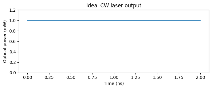
As expected for an ideal source, the output amplitude is a constant \(\sqrt{P}\), so the instantaneous power \(\lvert a \rvert^2\) stays at 1 mW.

time_step = 1e-12
num_steps = 2000
t = np.arange(num_steps) * time_step

time_stepper = laser.setup_time_stepper(time_step=time_step, carrier_frequency=f0)
output = time_stepper.step(steps=num_steps, time_step=time_step)
a = output["P0@0"]

fig, ax = plt.subplots(figsize=(7, 3), tight_layout=True)
ax.plot(t * 1e9, np.abs(a) ** 2 * 1e3)
ax.set(xlabel="Time (ns)", ylabel="Optical power (mW)", ylim=(0, 1.2))
_ = ax.set_title("Ideal CW laser output")

Laser Detuning

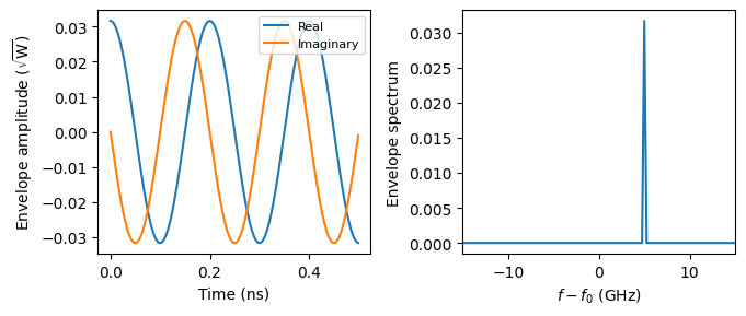
If the frequency argument is None (the default), the laser frequency equals the carrier frequency and the envelope is constant. Setting frequency to an absolute value detuned from the carrier by \(\Delta f\) makes the envelope rotate at that rate. PhotonForge uses the \(e^{-j 2 \pi f t}\) phasor convention for the physical field, so a laser at \(f_0 + \Delta f\) produces the envelope \(a(t) = \sqrt{P} \, e^{-j 2 \pi \Delta f t}\). When mapping an envelope spectrum computed with the standard FFT convention back to absolute optical frequencies, an envelope component at frequency \(f\) corresponds to the optical frequency \(f_0 - f\).

Below, the laser is detuned 5 GHz above the carrier: the envelope rotates with a 200 ps period and the spectrum shows a single tone at \(f - f_0 = 5\) GHz.

detuning = 5e9
laser_detuned = pfa.cw_laser(power=1e-3, frequency=f0 + detuning)

num_steps = 4000
t = np.arange(num_steps) * time_step

time_stepper = laser_detuned.setup_time_stepper(time_step=time_step, carrier_frequency=f0)
a = time_stepper.step(steps=num_steps, time_step=time_step)["P0@0"]

spectrum = np.abs(np.fft.fftshift(np.fft.fft(a))) / num_steps
freq_offset = -np.fft.fftshift(np.fft.fftfreq(num_steps, time_step))
order = np.argsort(freq_offset)

fig, (ax1, ax2) = plt.subplots(1, 2, figsize=(7, 3), tight_layout=True)
ax1.plot(t[:500] * 1e9, np.real(a[:500]), label="Real")
ax1.plot(t[:500] * 1e9, np.imag(a[:500]), label="Imaginary")
ax1.set(xlabel="Time (ns)", ylabel=r"Envelope amplitude ($\sqrt{\mathrm{W}}$)")
ax1.legend(loc="upper right", fontsize=8)
ax2.plot(freq_offset[order] / 1e9, spectrum[order])
ax2.set(xlabel="$f - f_0$ (GHz)", ylabel="Envelope spectrum", xlim=(-15, 15))

print(f"Spectral peak at {freq_offset[np.argmax(spectrum)] / 1e9:.1f} GHz")

Spectral peak at 5.0 GHz

Phase Noise and Linewidth

Real lasers have a finite spectral linewidth caused by spontaneous emission phase noise. The time stepper implements it as a discrete-time Wiener process: at each step, the phase receives an independent Gaussian increment with variance

\[\mathrm{Var}[\Delta \phi] = 2 \pi \, \Delta \nu \, \Delta t\]

where \(\Delta \nu\) is the linewidth argument, the full width at half maximum (FWHM) of the resulting Lorentzian field spectrum

\[S(f) \propto \frac{(\Delta \nu / 2)^2}{(f - f_\mathrm{laser})^2 + (\Delta \nu / 2)^2}\]

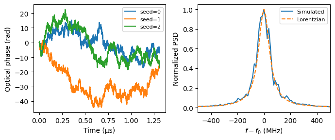
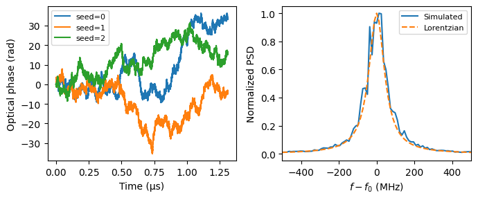
The seed argument makes each noise realization reproducible. We use a 100 MHz linewidth to keep the simulation short (single-frequency semiconductor lasers typically range from kHz to a few MHz) and check the two signatures of this noise model: the phase performs a random walk, and the averaged power spectrum of the field envelope follows the expected Lorentzian lineshape.

linewidth = 100e6
laser_pn = pfa.cw_laser(power=1e-3, linewidth=linewidth, seed=0)

time_step_pn = 1e-11
num_steps = 2**17
num_segments = 16
seg_len = num_steps // num_segments
t = np.arange(num_steps) * time_step_pn

fig, (ax1, ax2) = plt.subplots(1, 2, figsize=(7, 3), tight_layout=True)

spectrum = np.zeros(seg_len)
for seed in range(3):
    laser_pn.update(seed=seed)
    time_stepper = laser_pn.setup_time_stepper(
        time_step=time_step_pn, carrier_frequency=f0, show_progress=False
    )
    a = time_stepper.step(steps=num_steps, time_step=time_step_pn, show_progress=False)["P0@0"]
    ax1.plot(t * 1e6, np.unwrap(np.angle(a)), label=f"seed={seed}")
    for i in range(num_segments):
        seg = a[i * seg_len : (i + 1) * seg_len]
        spectrum += np.abs(np.fft.fftshift(np.fft.fft(seg))) ** 2
spectrum /= spectrum.max()

freq = np.fft.fftshift(np.fft.fftfreq(seg_len, time_step_pn))
lorentzian = 1 / (1 + (2 * freq / linewidth) ** 2)

crossings = freq[spectrum >= 0.5]
fwhm = crossings.max() - crossings.min()

ax1.set(xlabel="Time (µs)", ylabel="Optical phase (rad)")
ax1.legend(fontsize=8)
ax2.plot(freq / 1e6, spectrum, label="Simulated")
ax2.plot(freq / 1e6, lorentzian, "--", label="Lorentzian")
ax2.set(xlabel="$f - f_0$ (MHz)", ylabel="Normalized PSD", xlim=(-500, 500))
ax2.legend(fontsize=8)

print(f"Measured FWHM: {fwhm / 1e6:.0f} MHz (specified: {linewidth / 1e6:.0f} MHz)")

Measured FWHM: 98 MHz (specified: 100 MHz)

Relative Intensity Noise

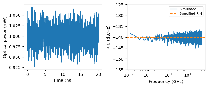
Power fluctuations of a laser are characterized by the relative intensity noise power spectral density, \(\mathrm{RIN}(f) = S_{\delta P}(f) / P_0^2\), with units of 1/Hz and usually quoted in dB/Hz. The rel_intensity_noise argument sets a one-sided white RIN PSD: at each time step, the power receives an independent Gaussian fluctuation with variance

\[\mathrm{Var}[P] = \mathrm{RIN} \, \frac{P_0^2}{2 \, \Delta t}\]

which corresponds to the specified PSD band-limited by the Nyquist frequency of the simulation (the power is also clamped at zero). Typical semiconductor lasers show RIN levels between \(-160\) and \(-130\) dB/Hz. We configure \(-140\) dB/Hz and verify that the one-sided PSD of the simulated relative power fluctuations is white at the specified level.

rin_db = -140
laser_rin = pfa.cw_laser(power=1e-3, rel_intensity_noise=10 ** (rin_db / 10), seed=0)

time_stepper = laser_rin.setup_time_stepper(
    time_step=time_step_pn, carrier_frequency=f0, show_progress=False
)
a = time_stepper.step(steps=num_steps, time_step=time_step_pn, show_progress=False)["P0@0"]
power = np.abs(a) ** 2

psd = np.zeros(seg_len // 2 + 1)
for i in range(num_segments):
    seg = power[i * seg_len : (i + 1) * seg_len]
    psd += 2 * np.abs(np.fft.rfft(seg - seg.mean())) ** 2 * time_step_pn / seg_len
psd /= num_segments * power.mean() ** 2
freq = np.fft.rfftfreq(seg_len, time_step_pn)

fig, (ax1, ax2) = plt.subplots(1, 2, figsize=(7, 3), tight_layout=True)
ax1.plot(t[:2000] * 1e9, power[:2000] * 1e3)
ax1.set(xlabel="Time (ns)", ylabel="Optical power (mW)")
ax2.semilogx(freq[1:] / 1e9, 10 * np.log10(psd[1:]), label="Simulated")
ax2.axhline(rin_db, color="tab:orange", linestyle="--", label="Specified RIN")
ax2.set(xlabel="Frequency (GHz)", ylabel="RIN (dB/Hz)", ylim=(rin_db - 15, rin_db + 15))
ax2.legend(fontsize=8)

print(f"Measured RIN: {10 * np.log10(psd[1:].mean()):.1f} dB/Hz (specified: {rin_db} dB/Hz)")

Measured RIN: -140.0 dB/Hz (specified: -140 dB/Hz)

Laser Noise at a Detector

Abstract components can be wired into circuits like any other PhotonForge component. Here we connect the laser to a photodiode with responsivity \(R = 0.8\) A/W and compare the detected signal with the laser RIN disabled and enabled. The photodiode outputs the voltage \(V = G R P\), where \(G\) is the transimpedance gain (1 V/A by default), converted to an electrical wave amplitude \(V / \sqrt{Z_0}\) at its port.

The photodiode model generates its own shot noise, with a relative PSD of \(2 q / (R P_0)\), about \(-154\) dB/Hz at the detected power in this link. This sets the noise floor of the ideal link, while the laser RIN of \(-140\) dB/Hz sits 14 dB above it and dominates the detected noise. Since the parametric update method modifies the laser in place, the same circuit can be re-simulated with new laser parameters without rebuilding it.

responsivity = 0.8
z0 = 50.0
laser_link = pfa.cw_laser(power=1e-3)
photodiode = pfa.photodiode(responsivity=responsivity, seed=7)

link = pf.Component("detection_link")
laser_ref = link.add_reference(laser_link)
photodiode_ref = link.add_reference(photodiode)
photodiode_ref.connect("P0", laser_ref["P0"])
link.add_port(photodiode_ref["E0"])
link.add_model(pf.CircuitModel(), "Circuit")

voltages = {}
for label, rin in [("Ideal laser", 0), ("Laser with RIN", 10 ** (rin_db / 10))]:
    laser_link.update(rel_intensity_noise=rin, seed=3)
    time_stepper = link.setup_time_stepper(
        time_step=time_step_pn, carrier_frequency=f0, show_progress=False
    )
    output = time_stepper.step(steps=num_steps, time_step=time_step_pn, show_progress=False)
    voltages[label] = np.real(output["E0@0"]) * np.sqrt(z0)

q_e = 1.602176634e-19
shot_db = 10 * np.log10(2 * q_e / (responsivity * 1e-3))

fig, (ax1, ax2) = plt.subplots(1, 2, figsize=(7, 3), tight_layout=True)
for label, v in voltages.items():
    ax1.plot(t[:2000] * 1e9, v[:2000] * 1e3, label=label, alpha=0.8)
    psd = np.zeros(seg_len // 2 + 1)
    for i in range(num_segments):
        seg = v[i * seg_len : (i + 1) * seg_len]
        psd += 2 * np.abs(np.fft.rfft(seg - seg.mean())) ** 2 * time_step_pn / seg_len
    psd /= num_segments * v.mean() ** 2
    ax2.semilogx(freq[1:] / 1e9, 10 * np.log10(psd[1:]), label=label, alpha=0.8)
    print(f"{label}: detected noise PSD {10 * np.log10(psd[1:].mean()):.1f} dB/Hz")

ax1.set(xlabel="Time (ns)", ylabel="Detected voltage (mV)")
ax1.legend(fontsize=8)
ax2.axhline(rin_db, color="k", linestyle="--", linewidth=1, label="Laser RIN")
ax2.axhline(shot_db, color="k", linestyle=":", linewidth=1, label="Shot noise floor")
ax2.set(xlabel="Frequency (GHz)", ylabel="Relative noise PSD (dB/Hz)", ylim=(-160, -130))
_ = ax2.legend(fontsize=8, loc="upper left")

Ideal laser: detected noise PSD -154.0 dB/Hz
Laser with RIN: detected noise PSD -139.8 dB/Hz

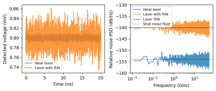
The detected noise matches the expected levels: the ideal-laser link is limited by the photodiode shot noise near \(-154\) dB/Hz, and enabling the laser RIN raises the detected noise to the configured \(-140\) dB/Hz.

Summary

• The CW laser is the basic optical source for time-domain simulations: create it with pfa.cw_laser, initialize with setup_time_stepper (time step and carrier frequency), and run with step.

• Optical envelope amplitudes are in \(\sqrt{\mathrm{W}}\), so \(\lvert a \rvert^2\) is the instantaneous power; the mean power is set by power.

• frequency sets the absolute laser frequency: detuning from the carrier by \(\Delta f\) rotates the envelope as \(e^{-j 2 \pi \Delta f t}\).

• linewidth adds Wiener phase noise producing a Lorentzian line with the specified FWHM, and rel_intensity_noise adds a white one-sided RIN PSD; seed makes noise realizations reproducible.

• Sources combine with modulators, waveguides, and detectors from the abstract module for circuit-level studies. For a directly modulated laser with rate-equation dynamics, see DMLaserTimeStepper, and to add optical noise to any existing signal, see OpticalNoiseTimeStepper.