Optical Noise

The OpticalNoiseTimeStepper is a white optical noise source: at every time step it emits an independent, zero-mean, circularly symmetric complex Gaussian sample. Its single parameter is the one-sided amplitude spectral density noise (in \(\sqrt{\mathrm{W} / \mathrm{Hz}}\)).

Two situations call for a standalone noise source. The first is noise loading: adding a calibrated amount of noise to a signal to set a known optical signal-to-noise ratio (OSNR), the standard way to measure receiver sensitivity. The second is replacing the accumulated amplified spontaneous emission (ASE) of a multi-amplifier line with a single equivalent source instead of simulating every amplifier.

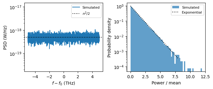
In the simulated spectral slice of width \(1 / \Delta t\), the emitted field has a flat power spectral density of \(n^2 / 2\) and a total power of \(n^2 / (2 \Delta t)\): as with the ASE of the OpticalAmplifierTimeStepper, the time step sets the bandwidth over which the white noise is realized.

This guide shows how to use the source: first standalone, relating its output to the noise parameter, then in its main role, loading a carrier to a target OSNR and degrading the eye of a data signal in controlled steps.

Setup

import matplotlib.pyplot as plt
import numpy as np
import photonforge as pf
import photonforge.abstract as pfa

viewer = pf.live_viewer.LiveViewer()

LiveViewer started at http://localhost:65341

tech = pf.basic_technology()
pf.config.default_technology = tech

f0 = pf.C_0 / 1.55  # optical carrier at 1.55 um
time_step = 0.1e-12  # 0.1 ps step -> 10 THz simulated noise bandwidth

Noise Statistics

The abstract optical_noise component is a source with a single optical port, so it runs standalone like the lasers. Two statistical signatures characterize it. The spectrum of the emitted field is flat at \(n^2 / 2\) across the whole simulated band. And because the field samples are circularly symmetric Gaussians, the instantaneous power \(\lvert a \rvert^2\) follows an exponential distribution with mean \(n^2 / (2 \Delta t)\), the same statistics as unpolarized thermal light or pure ASE.

asd = 1e-9  # amplitude spectral density n (sqrt(W/Hz)); the seed makes the run reproducible
source = pfa.optical_noise(noise=asd, seed=0)
viewer(source)

# Run the source standalone and collect a long noise record
num_steps = 2**16
time_stepper = source.setup_time_stepper(
    time_step=time_step, carrier_frequency=f0, show_progress=False
)
a = time_stepper.step(steps=num_steps, time_step=time_step, show_progress=False)["P0@0"]
power = np.abs(a) ** 2  # instantaneous power of the emitted field

# Segment-averaged PSD of the emitted field
num_segments = 16
seg_len = num_steps // num_segments
psd = np.zeros(seg_len)
for k in range(num_segments):
    seg = a[k * seg_len : (k + 1) * seg_len]
    psd += np.abs(np.fft.fftshift(np.fft.fft(seg))) ** 2 * time_step / seg_len
psd /= num_segments
freq = np.fft.fftshift(np.fft.fftfreq(seg_len, time_step))

mean_power = asd**2 / (2 * time_step)  # expected total power n^2 / (2 dt)

fig, (ax1, ax2) = plt.subplots(1, 2, figsize=(7, 3), tight_layout=True)
ax1.semilogy(freq / 1e12, psd, label="Simulated")
ax1.axhline(asd**2 / 2, color="k", linestyle=":", label="$n^2 / 2$")
ax1.set(xlabel="$f - f_0$ (THz)", ylabel="PSD (W/Hz)", ylim=(asd**2 / 60, asd**2 * 15))
ax1.legend(fontsize=8)
# Histogram of the normalized power against the exponential distribution
ax2.hist(power / mean_power, bins=60, density=True, alpha=0.7, label="Simulated")
x = np.linspace(0, 8, 200)
ax2.plot(x, np.exp(-x), "k:", label="Exponential")
ax2.set(xlabel="Power / mean", ylabel="Probability density", yscale="log")
ax2.legend(fontsize=8)

print(f"Mean power: {power.mean() * 1e6:.3f} µW (n²/2Δt = {mean_power * 1e6:.3f} µW)")

Mean power: 5.013 µW (n²/2Δt = 5.000 µW)

Loading a Carrier to a Target OSNR

The most common job for a noise source is noise loading: setting a known optical signal-to-noise ratio to characterize how a receiver or a link degrades. OSNR is conventionally quoted in a 0.1 nm (12.5 GHz) reference bandwidth, so for a signal power \(P\) the required noise ASD is

\[\mathrm{OSNR} = \frac{P}{(n^2 / 2) B_\mathrm{ref}} \quad \Rightarrow \quad n = \sqrt{\frac{2 P}{\mathrm{OSNR} \cdot B_\mathrm{ref}}}\]

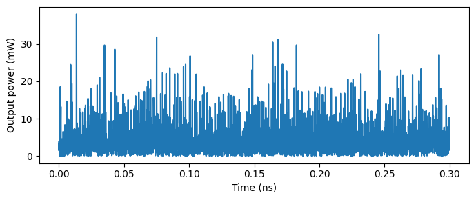
We combine a 1 mW carrier with the calibrated noise in a 3 dB directional_coupler, which attenuates signal and noise equally and therefore preserves the ratio, and measure the OSNR back from the output field.

p_signal = 1e-3
target_osnr_db = 20.0
b_ref = 12.5e9  # conventional 0.1 nm OSNR reference bandwidth

# Noise ASD required for the target OSNR: n = sqrt(2 P / (OSNR * B_ref))
asd_load = np.sqrt(2 * p_signal / (10 ** (target_osnr_db / 10) * b_ref))

# Combine the carrier and the noise in a 3 dB coupler; the unused arm is terminated
link = pf.Component("osnr_link")
laser_ref = link.add_reference(pfa.cw_laser(power=p_signal))
noise_ref = link.add_reference(pfa.optical_noise(noise=asd_load, seed=1))
coupler_ref = link.add_reference(pfa.directional_coupler())
termination_ref = link.add_reference(pfa.optical_termination())
laser_ref.connect("P0", coupler_ref["P0"])
noise_ref.connect("P0", coupler_ref["P1"])
termination_ref.connect("P0", coupler_ref["P3"])
link.add_port(coupler_ref["P2"], "out")
link.add_model(pf.CircuitModel(), "Circuit")

time_stepper = link.setup_time_stepper(
    time_step=time_step, carrier_frequency=f0, show_progress=False
)
a = time_stepper.step(steps=num_steps, time_step=time_step, show_progress=False)["out@0"]

# Signal power from the mean field, noise PSD from the fluctuations
signal_power = np.abs(a.mean()) ** 2
noise_psd = (np.abs(a - a.mean()) ** 2).mean() * time_step
osnr_measured = 10 * np.log10(signal_power / (noise_psd * b_ref))

fig, ax = plt.subplots(figsize=(7, 3), tight_layout=True)
t = np.arange(num_steps) * time_step
ax.plot(t[:3000] * 1e9, np.abs(a[:3000]) ** 2 * 1e3)
ax.set(xlabel="Time (ns)", ylabel="Output power (mW)")

print(f"Required noise ASD: {asd_load:.3e} sqrt(W/Hz)")
print(f"Measured OSNR in {b_ref / 1e9:.1f} GHz: {osnr_measured:.2f} dB (target {target_osnr_db:.1f} dB)")

Required noise ASD: 4.000e-08 sqrt(W/Hz)
Measured OSNR in 12.5 GHz: 20.00 dB (target 20.0 dB)

Noise-Loaded Eye Diagrams

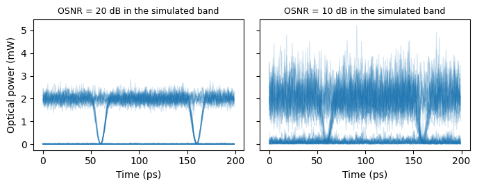
Loading a data signal instead of a carrier shows the OSNR penalty where it matters: in the eye. A 10 Gb/s NRZ transmitter (a mach_zehnder_modulator at quadrature driven by a PRBS pattern) is combined with the noise source.

Since an OSNR value is only meaningful together with its bandwidth, and the raw eye sees every bit of noise in the simulated band, here we quote the loading directly in the simulated bandwidth of \(1 / \Delta t = 1\) THz: signal-to-noise ratios of 20 dB and 10 dB in the slice, which correspond to 39 dB and 29 dB in the 12.5 GHz reference (the conversion is \(10 \log_{10}(B_\mathrm{sim} / B_\mathrm{ref}) = 19\) dB). In a receiver simulation, an optical band-pass filter in front of the detector would remove most of this out-of-band noise. Note the asymmetry between the rails: on the one level the noise beats against the signal field, so it appears amplified, while the zero level only carries the small noise-noise term, the same structure seen with amplifier ASE.

bit_rate = 10e9
time_step_eye = 1e-12
unit_interval = int(round(1 / bit_rate / time_step_eye))  # samples per bit
num_bits = 128
t_eye = np.arange(2 * unit_interval) * time_step_eye  # eye spans two unit intervals
v_pi = 4.0
z0 = 50.0

b_sim = 1 / time_step_eye  # simulated bandwidth in which the loading is quoted
fig, axes = plt.subplots(1, 2, figsize=(7, 2.8), sharey=True, tight_layout=True)
for ax, osnr_db in zip(axes, [20, 10]):
    # Loading quoted in the full simulated bandwidth
    asd_eye = np.sqrt(2 * p_signal / (10 ** (osnr_db / 10) * b_sim))
    # Laser power chosen so the average signal power at the output is p_signal
    # (the quadrature-biased NRZ averages to half, and the combiner halves again)
    transmitter = pf.Component("noisy_link")
    laser_ref = transmitter.add_reference(pfa.cw_laser(power=4 * p_signal))
    modulator_ref = transmitter.add_reference(
        pfa.mach_zehnder_modulator(v_pi=v_pi, phase_bias=90)
    )
    # NRZ drive swinging v_pi/2 around the quadrature point (amplitudes in V / sqrt(z0))
    source_ref = transmitter.add_reference(
        pfa.signal_source(
            frequency=bit_rate,
            amplitude=(v_pi / 2) / np.sqrt(z0),
            offset=(-v_pi / 4) / np.sqrt(z0),
            waveform="trapezoid",
            rise=0.1,
            fall=0.1,
            width=1.1,
            prbs=7,
            seed=0,
        )
    )
    # The sqrt(2) compensates the 3 dB the combiner takes from the noise path
    noise_ref = transmitter.add_reference(pfa.optical_noise(noise=asd_eye * np.sqrt(2), seed=2))
    coupler_ref = transmitter.add_reference(pfa.directional_coupler())
    termination_ref = transmitter.add_reference(pfa.optical_termination())
    # Chain in signal-flow order: laser -> MZM (driven by the source) -> combiner
    modulator_ref.connect("P0", laser_ref["P0"])
    source_ref.connect("E0", modulator_ref["E0"])
    coupler_ref.connect("P0", modulator_ref["P1"])
    noise_ref.connect("P0", coupler_ref["P1"])
    termination_ref.connect("P0", coupler_ref["P3"])
    transmitter.add_port(coupler_ref["P2"], "out")
    transmitter.add_model(pf.CircuitModel(), "Circuit")

    num_steps_eye = unit_interval * num_bits
    time_stepper = transmitter.setup_time_stepper(
        time_step=time_step_eye, carrier_frequency=f0, show_progress=False
    )
    output = time_stepper.step(steps=num_steps_eye, time_step=time_step_eye, show_progress=False)
    power = np.abs(output["out@0"]) ** 2

    # Fold the received power into two-unit-interval segments to form the eye
    segments = power[unit_interval // 2 :]
    segments = segments[: len(segments) // (2 * unit_interval) * 2 * unit_interval]
    for segment in segments.reshape(-1, 2 * unit_interval):
        ax.plot(t_eye * 1e12, segment * 1e3, color="C0", alpha=0.2, linewidth=0.8)
    ax.set_title(f"OSNR = {osnr_db} dB in the simulated band", fontsize=9)
    ax.set_xlabel("Time (ps)")
axes[0].set_ylabel("Optical power (mW)")
plt.show()

Summary

• pfa.optical_noise is a white-noise optical source: circularly symmetric complex Gaussian samples, independent at every time step, with the one-sided amplitude spectral density set by noise and reproducible realizations via seed.

• In the simulation, the envelope PSD is flat at \(n^2 / 2\) and the total emitted power is \(n^2 / (2 \Delta t)\): the time step sets the realized noise bandwidth, so quantitative comparisons should use spectral densities rather than raw powers.

• The instantaneous power is exponentially distributed, the statistics of thermal light and ASE.

• Noise loading to a target OSNR uses \(n = \sqrt{2 P / (\mathrm{OSNR} \cdot B_\mathrm{ref})}\) with the conventional 12.5 GHz (0.1 nm) reference bandwidth, and a balanced combiner preserves the ratio.

• On data signals the loaded noise produces the classic asymmetric eye, dominated by signal-noise beating on the one level; for noise tied to a gain element, use the OpticalAmplifierTimeStepper, and for multiplicative source noise, the RIN and linewidth of the CW Laser.