Verilog-A Export

TimeStepper.write_verilog_a writes a configured time stepper as one self-contained Verilog-A module. The time stepper can belong to a single component or to a whole circuit; for a circuit, every component is written into the same module. The exported photonic circuit can then be placed in a SPICE netlist next to the driver, the transimpedance amplifier and the rest of the electronics, so the complete transceiver is simulated in one circuit simulator.

This guide exports a Mach-Zehnder transmitter, laser included, compiles the module with OpenVAF-Reloaded and simulates it in ngspice with the same drive signal used in PhotonForge.

Compiler and simulator

The exported modules use the Verilog-A absdelay operator for propagation delays and white_noise for noise sources, and both the compiler and the simulator must implement them. This guide uses OpenVAF-Reloaded 23.6.0 and ngspice-46 from the Ngspice_OpenVAF_Enhancements repository, which provides prebuilt binaries for Windows, Linux and macOS in its bin/<platform>/<architecture> folders. Take both programs from the same folder and put it on the system path so that openvaf-r and ngspice are found.

import subprocess

import matplotlib.pyplot as plt
import numpy as np
import photonforge as pf
import photonforge.abstract as pfa
import siepic_forge as siepic
from scipy.ndimage import gaussian_filter1d

# SiEPIC EBeam silicon process, with its 500 nm strip waveguide as the default port
pf.config.default_technology = siepic.ebeam()
pf.config.default_kwargs = {"euler_fraction": 0.5, "port_spec": "TE_1550_500"}

viewer = pf.live_viewer.LiveViewer()

LiveViewer started at http://127.0.0.1:36715. Call its 'stop()' method to free the port.

Transmitter circuit

The transmitter is a Mach-Zehnder interferometer fed by a CW laser. One arm is a 2 mm silicon phase shifter with \(V_\pi L = 1.5\) V cm, so its half-wave voltage is \(V_\pi = 7.5\) V, and a 30 GHz electro-optic bandwidth. The other arm is a plain waveguide of the same length. Two s-bend directional couplers split and recombine the light.

The phase shifter is a straight waveguide with an electrode on either side and an electrical port E0 for the drive. Its behavior comes from AnalyticWaveguideModel, with a PhaseModTimeStepper attached for the time domain. The reference arm uses AnalyticWaveguideTimeStepper.

f_c = pf.C_0 / 1.55  # carrier frequency, pf.C_0 is in um/s
bit_rate = 10e9
time_step = 0.5e-12  # 200 samples per bit
z0 = 50.0  # reference impedance of the ports

# Waveguide shared by both arms
length = 2000.0  # um
waveguide = dict(
    n_eff=2.4,
    n_group=4.2,
    reference_frequency=f_c,
    length=length,
    propagation_loss=1e-4,  # dB/um, that is 1 dB/cm
)
v_pil = 1.5e4  # V um, that is 1.5 V cm
v_pi = v_pil / length  # 7.5 V


@pf.parametric_component
def phase_shifter(*, length=length):
    component = pf.parametric.straight(length=length)

    # Electrodes on the metal layer, 1.1 um from the waveguide center
    component.add(
        "M1_heater",
        pf.Rectangle((0, 1.1), (length, 1.9)),
        pf.Rectangle((0, -1.9), (length, -1.1)),
    )

    # Virtual electrical port for the drive, on the upper electrode
    component.add_port(
        pf.Port(
            (length / 2, 1.5),
            90,
            spec=pf.virtual_port_spec(classification="electrical"),
        )
    )

    # The time stepper attached to the model is what gets exported
    model = pf.AnalyticWaveguideModel(v_piL=v_pil, **waveguide)
    model.time_stepper = pf.PhaseModTimeStepper(v_piL=v_pil, f_3dB=30e9, **waveguide)
    component.add_model(model)
    return component


@pf.parametric_component
def reference_arm(*, length=length):
    # Same waveguide without the electro-optic effect; the delay is applied directly
    model = pf.AnalyticWaveguideModel(**waveguide)
    model.time_stepper = pf.AnalyticWaveguideTimeStepper(**waveguide)
    return pf.parametric.straight(length=length, model=model)


# 10 um s-bend offsets separate the two arms by 20 um
coupler = pf.parametric.s_bend_coupler(
    coupling_distance=0.6,
    coupling_length=4.7,
    s_bend_length=40,
    s_bend_offset=10,
    model=pf.DirectionalCouplerModel(),
)

# 1 mW laser, and a termination for the unused input of the first coupler
laser = pfa.cw_laser(power=1e-3, frequency=f_c)
termination = pfa.optical_termination()

The netlist places the arms and the second coupler with physical connections; the last pair of ports meets geometrically and closes the interferometer. The laser and the termination have no layout, so each is placed next to its coupler port and attached with a virtual connection. The circuit exposes three ports: the drive and the two optical outputs.

transmitter = pf.component_from_netlist(
    {
        "name": "Transmitter",
        "instances": {
            # Abstract blocks are built at the origin, so place them by their ports
            "laser": {"component": laser, "origin": (-20, 0)},
            "dump": {"component": termination, "origin": (-20, 20.6)},
            "dc0": coupler,
            "ref": reference_arm(),
            "arm": phase_shifter(),
            "dc1": coupler,
        },
        "connections": [
            (("ref", "P0"), ("dc0", "P2")),
            (("dc1", "P0"), ("ref", "P1")),
            (("arm", "P0"), ("dc0", "P3")),
        ],
        "virtual connections": [
            (("laser", "P0"), ("dc0", "P0")),
            (("dump", "P0"), ("dc0", "P1")),
        ],
        "ports": [
            ("arm", "E0", "DRIVE"),
            ("dc1", "P2", "OUT1"),
            ("dc1", "P3", "OUT2"),
        ],
        "models": [(pf.CircuitModel(), "Circuit")],
    }
)
viewer(transmitter)

LayoutSchematic

Simulation in PhotonForge

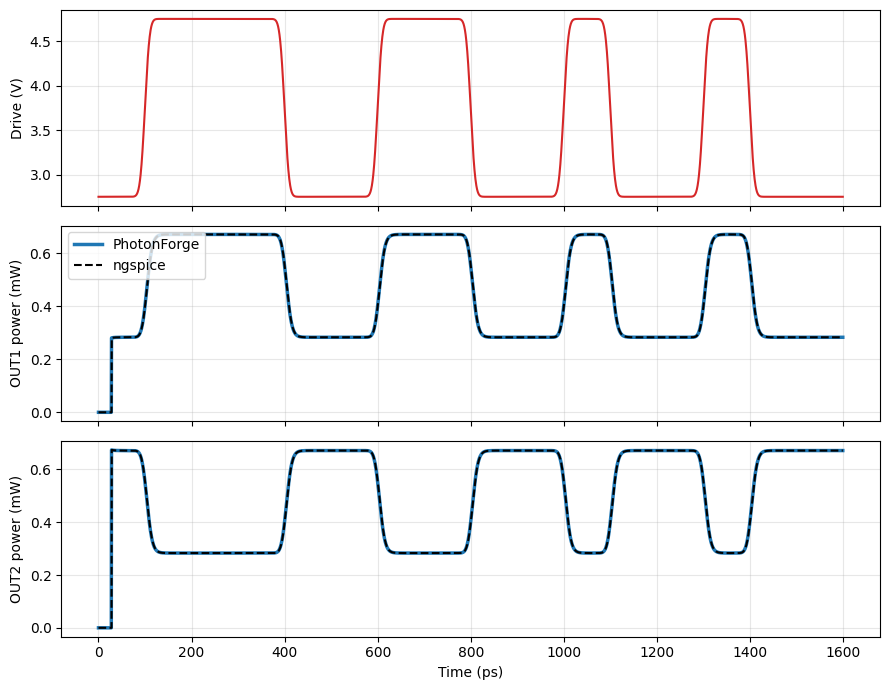
The drive is a 10 Gb/s non-return-to-zero (NRZ) pattern of 16 random bits with smoothed edges. It swings 2 V peak to peak around \(V_\pi / 2\), which biases the interferometer at quadrature. The electrical key of a matched port carries the voltage divided by \(\sqrt{z_0}\).

# 16 random bits, each held for one bit period, with edges of about 20 ps
rng = np.random.default_rng(1)
bits = rng.integers(0, 2, 16)
samples_per_bit = round(1 / (bit_rate * time_step))
time = time_step * np.arange(bits.size * samples_per_bit)
nrz = np.repeat(bits, samples_per_bit).astype(float)
nrz = gaussian_filter1d(nrz, sigma=8e-12 / time_step, mode="nearest")
volts = v_pi / 2 + 2.0 * (nrz - 0.5)

stepper = transmitter.setup_time_stepper(
    time_step=time_step, carrier_frequency=f_c, show_progress=False
)
inputs = pf.TimeSeries({"DRIVE@0": (volts / np.sqrt(z0)).astype(complex)}, time_step, 0)
stepper.reset()
outputs = stepper.step(inputs, show_progress=False)
photonforge_power = {
    key: np.abs(outputs.values[key]) ** 2 for key in ("OUT1@0", "OUT2@0")
}

Export to Verilog-A

One call writes the whole transmitter, laser and termination included, as a single module. The module name defaults to the file name, and the header of the file lists its terminals in order:

• each optical port becomes two terminals, _re and _im, for the real and imaginary parts of the field;

• each electrical port becomes one terminal;

• the last terminal, gnd, is the common reference.

source = stepper.write_verilog_a("transmitter.va")

# The header is the block of comment lines at the top of the file
header = [line for line in source.read_text().splitlines() if line.startswith("//")]
print("\n".join(header))

# "// Terminals: DRIVE_0, ..." becomes a list of names for the netlist
terminals = next(line for line in header if line.startswith("// Terminals:"))
terminals = terminals.split(": ")[1].split(", ")

// Generated by PhotonForge from a configured TimeStepper.
// Backend: openvaf
// Port convention: travelling_wave
// Time stepper: CircuitTimeStepper
// Keys: DRIVE@0, OUT1@0, OUT2@0
// Terminals: DRIVE_0, OUT1_0_re, OUT1_0_im, OUT2_0_re, OUT2_0_im, gnd
// Carrier frequency: 1.93414489032258062e+14 Hz
// Optical z0: 5.00000000000000000e+01 ohm
// Electrical DRIVE@0 z0: 5.00000000000000000e+01 ohm

OpenVAF compiles the source into transmitter.osdi, which ngspice loads directly.

# check=True raises an error if the compiler fails
subprocess.run(["openvaf-r", "transmitter.va"], check=True);

Finished building transmitter.va in 0.31s

Simulation in ngspice

Every terminal is a port with reference impedance \(z_0\). A voltage source of twice the drive voltage behind \(z_0\) launches the drive, and a resistor \(z_0\) to ground terminates each optical terminal; the output field is then the terminal voltage divided by \(\sqrt{z_0}\).

The OSDI model is loaded with pre_osdi and instantiated with a line starting with N. The maximum internal step is an eighth of the time step, so ngspice resolves the drive edges.

# One PWL vertex per sample, twice the voltage because the source sits behind z0
pwl = "\n".join(f"+ {t:.12e} {2 * v:.12e}" for t, v in zip(time, volts))

netlist = f"""* Mach-Zehnder transmitter driven by an NRZ pattern
.model tx transmitter
Vdrive drive 0 PWL(
{pwl}
+)
Rdrive drive DRIVE_0 {z0}
* Matched loads terminate both optical outputs
Rout1_re OUT1_0_re 0 {z0}
Rout1_im OUT1_0_im 0 {z0}
Rout2_re OUT2_0_re 0 {z0}
Rout2_im OUT2_0_im 0 {z0}
* The last terminal, gnd, goes to node 0
N1 {' '.join(terminals[:-1])} 0 tx
.tran {time_step / 8:.6e} {time[-1]:.6e} 0 {time_step / 8:.6e}
.control
pre_osdi transmitter.osdi
set numdgt=17
run
wrdata transmitter.txt v(OUT1_0_re) v(OUT1_0_im) v(OUT2_0_re) v(OUT2_0_im)
quit
.endc
.end
"""

with open("transmitter.cir", "w") as file:
    file.write(netlist)

# Batch mode, with the simulator messages written to a log file
subprocess.run(
    ["ngspice", "-b", "-o", "transmitter.log", "transmitter.cir"], check=True
);

******
** ngspice-46 : Circuit level simulation program
** Compiled with KLU Direct Linear Solver
** The U. C. Berkeley CAD Group
** Copyright 1985-1994, Regents of the University of California.
** Copyright 2001-2025, The ngspice team.
** Please get your ngspice manual from https://ngspice.sourceforge.io/docs.html
** Please file your bug-reports at http://ngspice.sourceforge.net/bugrep.html
** Creation Date: Fri Sep 11 18:11:56 UTC 2026
******

Batch mode

Comments and warnings go to log-file: transmitter.log

The output power is the sum of the squared real and imaginary terminal voltages divided by \(z_0\). The two outputs are complementary: the drive moves the interferometer about quadrature, and the power leaving one output is missing from the other.

# wrdata writes a time column before every vector, so each output takes four columns
data = np.loadtxt("transmitter.txt")
ngspice_power = {}
for index, key in enumerate(("OUT1@0", "OUT2@0")):
    column = 4 * index
    # ngspice picks its own time points, so interpolate onto the PhotonForge grid
    v_re = np.interp(time, data[:, column], data[:, column + 1])
    v_im = np.interp(time, data[:, column + 2], data[:, column + 3])
    ngspice_power[key] = (v_re**2 + v_im**2) / z0

fig, axes = plt.subplots(3, 1, figsize=(9, 7), sharex=True)
axes[0].plot(time * 1e12, volts, color="tab:red")
axes[0].set_ylabel("Drive (V)")
for ax, key in zip(axes[1:], ("OUT1@0", "OUT2@0")):
    ax.plot(time * 1e12, photonforge_power[key] * 1e3, lw=2.5, label="PhotonForge")
    ax.plot(time * 1e12, ngspice_power[key] * 1e3, "--", color="k", label="ngspice")
    ax.set_ylabel(f"{key[:4]} power (mW)")
axes[1].legend(loc="upper left")
axes[2].set_xlabel("Time (ps)")
for ax in axes:
    ax.grid(alpha=0.3)
fig.tight_layout()

Summary

• write_verilog_a writes a configured time stepper, from a single component or a full circuit, as one self-contained Verilog-A module. Configure it first with setup_time_stepper.

• The file header lists the module terminals in order: _re and _im pairs for optical ports, one terminal per electrical port, and gnd last.

• The module compiles with OpenVAF-Reloaded and runs in ngspice, where the transmitter reproduces the PhotonForge simulation and can be combined with the surrounding electronics.