Amplitude Modulator

The modulators covered so far are physics-based: an interferometer, a resonator, a phase shifter with a \(V_{\pi L}\). The AmplitudeModTimeStepper takes the opposite, behavioral approach: it maps the drive voltage to an optical amplitude scaling through a polynomial transfer function specified directly,

\[s_0 = a_0 + a_1 V + a_2 V^2 + a_3 V^3\]

which makes it the natural model for devices characterized by a measured transfer curve, such as electro-absorption modulators (EAMs), variable optical attenuators, or gain-modulated sections. The polynomial is scaled by the insertion loss and clipped to the physical envelope between the maximum transmission \(s_\mathrm{max} = 10^{-\mathrm{IL}/20}\) and the extinction floor \(s_\mathrm{max} 10^{-\mathrm{ER}/20}\). Amplitude-phase coupling is included through the chirp parameter \(C\),

\[\Delta \phi = C \ln \frac{s_\mathrm{total}}{s_\mathrm{max}}\]

and, as in the other electro-optic models, the drive voltage comes from the electrical port as \(V = \Re \lbrace A \rbrace \sqrt{Z_0}\), with voltage-dependent loss (dloss_dv) and a first-order electrical bandwidth (f_3dB) available.

This guide maps the static transfer and its clipping envelope, builds a model of a measured electro-absorption device, and looks at the chirp the modulator imprints on the light.

Setup

import matplotlib.pyplot as plt
import numpy as np
import photonforge as pf
import photonforge.abstract as pfa

viewer = pf.live_viewer.LiveViewer()

LiveViewer started at http://localhost:54100

tech = pf.basic_technology()
pf.config.default_technology = tech

f0 = pf.C_0 / 1.55
z0 = 50.0
time_step = 1e-12
p_laser = 1e-3

Static Transfer and Clipping

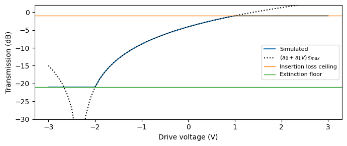
The abstract amplitude_modulator has two optical ports and the electrical drive E0. A modulator with \(s_0 = 0.7 + 0.3 V\), 1 dB insertion loss, and 20 dB extinction ratio illustrates all three regimes of the transfer function: the polynomial region in between, the insertion-loss ceiling where \(s_0 > 1\), and the extinction floor where the polynomial would drop below (or cross) zero.

Since both optical and electrical inputs can be injected together as a TimeSeries keyed by the component’s ports, the component is characterized directly, with no circuit around it: a constant optical field on P0 and a DC voltage on E0.

modulator = pfa.amplitude_modulator(a0=0.7, a1=0.3, insertion_loss=1, extinction_ratio=20)
viewer(modulator)

num_steps = 200
voltages = np.linspace(-3, 3, 61)
transmission = []
for voltage in voltages:
    # Run the time stepper directly on the modulator (no circuit needed)
    time_stepper = modulator.setup_time_stepper(
        time_step=time_step, carrier_frequency=f0, show_progress=False
    )
    # Inject a constant optical field on P0 and the DC voltage on E0 together
    inputs = pf.TimeSeries(
        {"P0@0": np.full(num_steps, np.sqrt(p_laser), complex),
         "E0@0": np.full(num_steps, voltage / np.sqrt(z0))},
        time_step,
    )
    out = time_stepper.step(inputs=inputs, show_progress=False)["P1@0"]
    # Steady-state power transmission at this bias
    transmission.append(np.abs(out[-1]) ** 2 / p_laser)
transmission = np.array(transmission)

# Maximum amplitude scaling allowed by the insertion loss
s_max = 10 ** (-1 / 20)
fig, ax = plt.subplots(figsize=(7, 3), tight_layout=True)
ax.plot(voltages, 10 * np.log10(transmission), label="Simulated")
ax.plot(voltages, 20 * np.log10(np.abs(0.7 + 0.3 * voltages) * s_max), "k:",
        label="$(a_0 + a_1 V) \\, s_{max}$")
ax.axhline(-1, color="C1", linewidth=1, label="Insertion loss ceiling")
ax.axhline(-21, color="C2", linewidth=1, label="Extinction floor")
ax.set(xlabel="Drive voltage (V)", ylabel="Transmission (dB)", ylim=(-30, 2))
_ = ax.legend(fontsize=8)

Modeling a Measured Device

The polynomial coefficients are usually not designed but fitted: the datasheet or a measurement gives the transfer curve, and the model reproduces it. As an example, we take the transmission of an electro-absorption modulator measured over its 0 to \(-3\) V operating range, fit a cubic polynomial to the field amplitude with numpy.polyfit, and hand the coefficients to the model.

# Measured EAM transmission (dB) over the operating range
v_measured = np.linspace(-3, 0, 13)
t_measured_db = -1 - 14 / (1 + np.exp(3.0 * (v_measured + 1.6)))

# The model polynomial acts on the FIELD AMPLITUDE, so convert from dB and
# fit the amplitude, not the dB transmission
amplitude_measured = 10 ** (t_measured_db / 20)
a3, a2, a1, a0 = np.polyfit(v_measured, amplitude_measured, 3)
eam = pfa.amplitude_modulator(a0=a0, a1=a1, a2=a2, a3=a3)

# Re-measure the fitted model over the operating range for comparison
voltages = np.linspace(-3, 0, 61)
transmission = []
for voltage in voltages:
    time_stepper = eam.setup_time_stepper(
        time_step=time_step, carrier_frequency=f0, show_progress=False
    )
    inputs = pf.TimeSeries(
        {"P0@0": np.full(num_steps, np.sqrt(p_laser), complex),
         "E0@0": np.full(num_steps, voltage / np.sqrt(z0))},
        time_step,
    )
    out = time_stepper.step(inputs=inputs, show_progress=False)["P1@0"]
    transmission.append(np.abs(out[-1]) ** 2 / p_laser)

fig, ax = plt.subplots(figsize=(7, 3), tight_layout=True)
ax.plot(v_measured, t_measured_db, "o", label="Measured")
ax.plot(voltages, 10 * np.log10(transmission), label="Cubic polynomial model")
ax.set(xlabel="Drive voltage (V)", ylabel="Transmission (dB)")
_ = ax.legend(fontsize=8)

print("Fitted coefficients: "
      f"a0 = {a0:.4f}, a1 = {a1:.4f} /V, a2 = {a2:.4f} /V², a3 = {a3:.4f} /V³")

Fitted coefficients: a0 = 0.8791, a1 = -0.0970 /V, a2 = -0.3849 /V², a3 = -0.0927 /V³

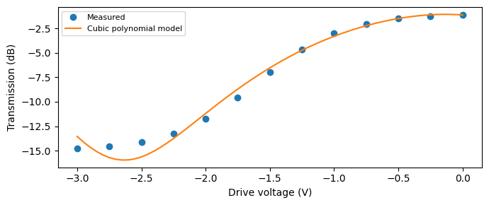
Note that the fit is performed on the field amplitude, where the model is polynomial, so the small residuals concentrate at deep extinction, where the logarithmic dB scale magnifies tiny amplitude errors; a fourth-order term or an extinction-ratio clamp tightens that region if it matters for the application.

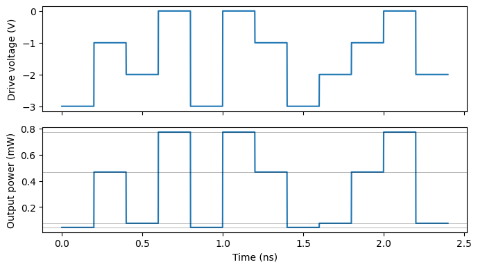
The nonlinear transfer matters most for multilevel signaling. Driving the fitted device with a four-level (PAM4) pattern whose electrical levels are equally spaced produces optical levels that are clearly not: the upper levels bunch together where the transfer curve flattens. This is exactly why real PAM4 transmitters pre-distort their drive levels.

# Equally spaced PAM4 electrical levels spanning the measured range
pam4_levels = np.linspace(-3, 0, 4)
symbol_sequence = pam4_levels[[0, 2, 1, 3, 0, 3, 2, 0, 1, 2, 3, 1]]

# Hold each symbol for 200 ps (5 GBd) and build the drive waveform
samples_per_symbol = 200
v_drive = np.repeat(symbol_sequence, samples_per_symbol)
num_steps = len(v_drive)
t = np.arange(num_steps) * time_step

# Constant optical input and the PAM4 drive, injected directly into the device
time_stepper = eam.setup_time_stepper(
    time_step=time_step, carrier_frequency=f0, show_progress=False
)
inputs = pf.TimeSeries(
    {"P0@0": np.full(num_steps, np.sqrt(p_laser), complex),
     "E0@0": v_drive / np.sqrt(z0)},
    time_step,
)
power = np.abs(time_stepper.step(inputs=inputs, show_progress=False)["P1@0"]) ** 2

# Steady-state optical power of each of the four levels, for the level markers
level_power = []
for level in pam4_levels:
    idx = np.nonzero(v_drive == level)[0]
    level_power.append(power[idx[-1]])

fig, (ax1, ax2) = plt.subplots(2, 1, figsize=(7, 4), sharex=True, tight_layout=True)
ax1.plot(t * 1e9, v_drive)
ax1.set_ylabel("Drive voltage (V)")
ax2.plot(t * 1e9, power * 1e3)
for p_level in level_power:
    ax2.axhline(p_level * 1e3, color="k", linewidth=0.5, alpha=0.4)
ax2.set(xlabel="Time (ns)", ylabel="Output power (mW)")

print("Electrical level spacing (V):", np.round(np.diff(pam4_levels), 2))
print("Optical level spacing (µW):  ", np.round(np.diff(np.array(level_power)) * 1e6, 1))

Electrical level spacing (V): [1. 1. 1.]
Optical level spacing (µW):   [ 31.8 391.9 305. ]

Chirp

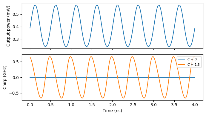
Absorption changes drag the refractive index with them (Kramers-Kronig again), so real amplitude modulators also modulate the optical phase. The chirp parameter ties the phase to the logarithm of the amplitude scaling, \(\Delta \phi = C \ln (s_\mathrm{total} / s_\mathrm{max})\), so the instantaneous frequency spikes at the transitions where the amplitude changes fastest.

We drive the first modulator with a sine and read both the power and the instantaneous frequency \(\Delta f = (\mathrm{d} \phi / \mathrm{d} t) / 2 \pi\) of the output envelope for a chirp-free and a chirped device.

drive_freq = 2e9
num_steps = 4000
t = np.arange(num_steps) * time_step
# Sinusoidal drive around the zero-volt bias point
v_drive = 0.5 * np.sin(2 * np.pi * drive_freq * t)

fig, (ax1, ax2) = plt.subplots(2, 1, figsize=(7, 4), sharex=True, tight_layout=True)
for chirp in [0, 1.5]:
    # Same modulator as the first section, with and without amplitude-phase coupling
    modulator_chirp = pfa.amplitude_modulator(
        a0=0.7, a1=0.3, insertion_loss=1, extinction_ratio=20, chirp=chirp
    )
    time_stepper = modulator_chirp.setup_time_stepper(
        time_step=time_step, carrier_frequency=f0, show_progress=False
    )
    inputs = pf.TimeSeries(
        {"P0@0": np.full(num_steps, np.sqrt(p_laser), complex),
         "E0@0": v_drive / np.sqrt(z0)},
        time_step,
    )
    out = time_stepper.step(inputs=inputs, show_progress=False)["P1@0"]
    # Instantaneous frequency of the output envelope (the chirp)
    frequency_offset = np.gradient(np.unwrap(np.angle(out)), time_step) / (2 * np.pi)
    if chirp == 0:
        # The power waveform is identical for both cases; plot it once
        ax1.plot(t * 1e9, np.abs(out) ** 2 * 1e3, color="C0")
    ax2.plot(t * 1e9, frequency_offset / 1e9, label=f"$C$ = {chirp}")

ax1.set_ylabel("Output power (mW)")
ax2.set(xlabel="Time (ns)", ylabel="Chirp (GHz)")
_ = ax2.legend(fontsize=8)

Summary

• pfa.amplitude_modulator is the behavioral electro-optic modulator: the voltage-to-amplitude map is the polynomial \(a_0 + a_1 V + a_2 V^2 + a_3 V^3\), scaled by the insertion loss and clipped between the IL ceiling and the ER floor.

• Polynomial coefficients are naturally obtained by fitting a measured transfer curve (fit the field amplitude, not the dB transmission), which makes the model a direct container for datasheet or measurement data.

• chirp couples amplitude to phase as \(C \ln(s_\mathrm{total} / s_\mathrm{max})\), producing the transient chirp of absorption-based modulators; dloss_dv and f_3dB behave as in the PhaseModTimeStepper.

• A lone component is characterized without any circuit: optical and electrical inputs are injected together as a TimeSeries keyed by its own port names.

• For physics-based modulators, see the interferometric MZMTimeStepper and the PhaseModTimeStepper; this model complements them whenever the device is known by its measured response.