Thermal Stabilization of Microring Resonators

The thermo-optic coefficient of silicon, \(dn/dT \approx 1.8 \times 10^{-4}\ \mathrm{K}^{-1}\), shifts a microring resonance by roughly 10 GHz per kelvin near 1550 nm. High-speed microring devices have linewidths of a few tens of gigahertz, so ambient temperature changes of a single kelvin detune them by a full linewidth. Practical microring links therefore run closed-loop: an integrated heater tunes the resonance, a monitor photodiode senses where the resonance sits, and a feedback controller holds it in place [1-3].

This example builds three such control loops around a time-domain microring model. The controllers are assembled from stock electrical blocks, with no custom time steppers: photodiode, adder, integrator, filter, and multiplier.

1. Flank lock: an integral controller holds the transmission of a passive ring at a setpoint on the resonance flank and rejects a thermal disturbance.

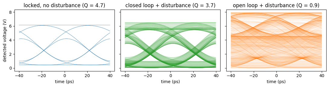
2. Mean-power lock of a modulator: the ring becomes a 25 Gb/s on-off-keyed modulator, and the loop stabilizes its mean output power, the scheme demonstrated by Padmaraju et al. [1]. Eye diagrams show the link surviving a thermal disturbance that destroys it open-loop.

3. Dither lock: a small dither tone and a lock-in error signal hold the ring exactly on resonance, the extremum where flank locking is blind, following [2].

Each loop is also integrated as a low-order ordinary differential equation, plotted for comparison with the circuit simulation.

The slow thermal response of the heater is the central constraint in this problem, and it is in the model: every loop below drives the ring through an explicit RC filter standing in for the heater’s thermal mass, this pole limits every loop bandwidth, and the controllers are designed against it, with a crossover at one third of the thermal pole. One idealization is made on top. Physical heaters respond in microseconds, while the optical time step is 0.1 ps, so a physical lock acquisition would take more than \(10^8\) steps; the thermal pole is therefore compressed to 30 MHz, and all other slow frequencies, the filters, gains, and disturbances, scale with it. Closed-loop behavior depends only on these ratios while the optics responds quasi-statically on loop timescales, which holds by orders of magnitude here (4 ps photon lifetime against nanoseconds) and even more so physically (4 ps against microseconds). Results map to physical scale by dividing the sub-linewidth frequencies and gains by one common factor and stretching the time axes by the same factor: with a 100 kHz heater bandwidth (1.6 us thermal time constant, a factor of 300), the 100 ns lock acquisition reads as 30 us, and the rejected 2 MHz disturbance maps to a 7 kHz ambient fluctuation, the regime of the cited experiments [1-3]. The fast side of the problem, the 25 Gb/s data and the cavity dynamics, is simulated at physical scale; compression narrows the gap between the data rate and the loop bandwidth, so the data-averaging task of the mean-power lock is harder here than in a physical system.

References

1. Padmaraju, K., Chan, J., Chen, L., Lipson, M., and Bergman, K. “Thermal stabilization of a microring modulator using feedback control.” Optics Express 2012 20 (27), 27999-28008, doi: 10.1364/OE.20.027999.

2. Padmaraju, K., Logan, D. F., Shiraishi, T., Ackert, J. J., Knights, A. P., and Bergman, K. “Wavelength locking and thermally stabilizing microring resonators using dithering signals.” Journal of Lightwave Technology 2014 32 (3), 505-512, doi: 10.1109/JLT.2013.2294564.

3. Padmaraju, K., and Bergman, K. “Resolving the thermal challenges for silicon microring resonator devices.” Nanophotonics 2014 3 (4-5), 269-281, doi: 10.1515/nanoph-2013-0013.

import matplotlib.pyplot as plt
import numpy as np
from scipy import signal
from scipy.integrate import solve_ivp

import photonforge as pf
import photonforge.abstract as pfa

viewer = pf.live_viewer.LiveViewer()

LiveViewer started at http://localhost:62265

tech = pf.basic_technology()
pf.config.default_technology = tech

z0 = 50.0  # impedance of the virtual electrical ports
sq = np.sqrt(z0)  # electrical wave amplitudes are V / sqrt(z0)
dt = 1e-13  # time step (s)

A Heater-Tunable Microring

The device under control is an all-pass microring from the abstract ring_resonator, based on the RingTimeStepper:

• 50 um circumference and group index 4.2, which gives a 1.43 THz free spectral range; the exact length is chosen so one round trip is an integer number of time steps;

• field coupling 0.4 to the bus, with the propagation loss set for critical coupling, so the on-resonance transmission drops to zero and the flanks are steep;

• a linear heater actuation dn_dv of \(10^{-3}\ \mathrm{V}^{-1}\), equivalent to about 5.5 K of local heating per volt through the silicon thermo-optic coefficient (the quadratic dependence of heater power on drive voltage is available through dn_dv2, but a linearized actuation keeps the loop analysis transparent);

• f_3dB = 0: the heater thermal low-pass is modeled as an explicit RC filter block in the loop, where it is visible and measurable.

The ring, and every other component in this example, is instantiated once and then referenced by all the circuits that use it.

The cold resonance is located from the frequency response, and the laser is parked 1.5 linewidths below it. Heating always lowers the resonance frequency, so the controller can pull the resonance down toward the laser but never push it up: heaters only heat, a constraint that reappears later as the integrator limits.

# ring geometry: one round trip = 7 time steps exactly
n_eff = 2.4
n_group = 4.2
length = 7 * dt * pf.C_0 / n_group  # um (pf.C_0 is in um/s)
fsr = pf.C_0 / (n_group * length)  # free spectral range (Hz)

# critical coupling: round-trip amplitude equals the coupler through coefficient
kappa = 0.4  # field coupling to the bus
t_c = np.sqrt(1 - kappa**2)  # coupler through coefficient
loss_db_um = -20 * np.log10(t_c) / length  # dB/um that makes a = t_c

dn_dv = 1e-3  # heater actuation (1/V), linearized

# the single ring instance used by every circuit in this example
ring = pfa.ring_resonator(
    kappa1=kappa, n_eff=n_eff, n_group=n_group, length=length,
    propagation_loss=loss_db_um, dn_dv=dn_dv, f_3dB=0, z0=z0,
)

# cold-ring frequency response over one free spectral range
freqs = np.linspace(pf.C_0 / 1.55 - 0.6 * fsr, pf.C_0 / 1.55 + 0.6 * fsr, 6001)
s = ring.s_matrix(freqs, show_progress=False)
t_f = np.abs(s[("P0@0", "P1@0")]) ** 2  # power transmission input -> through

# resonance = transmission minimum; linewidth from the half-transmission crossings
i_res = np.argmin(t_f)
f_res0 = freqs[i_res]
half = (t_f.max() + t_f.min()) / 2
left = i_res - np.argmax(t_f[i_res::-1] > half)  # crossing below the resonance
right = i_res + np.argmax(t_f[i_res:] > half)  # crossing above the resonance
fwhm = freqs[right] - freqs[left]

# heater tuning rate: dn raises n_eff, so the resonance moves DOWN in frequency
df_dv = f_res0 * dn_dv / n_group  # Hz per volt

# laser parked 1.5 linewidths below the cold resonance
f_laser = f_res0 - 1.5 * fwhm

print(f"resonance {f_res0 / 1e12:.4f} THz, FWHM {fwhm / 1e9:.1f} GHz "
      f"(loaded Q = {f_res0 / fwhm:.0f}), tuning rate {df_dv / 1e9:.1f} GHz/V")

fig, ax = plt.subplots(figsize=(7, 3), tight_layout=True)
ax.plot((freqs - f_res0) / 1e9, t_f)
ax.axvline((f_laser - f_res0) / 1e9, color="crimson", ls="--", lw=1, label="laser")
ax.set_xlim(-400, 400)
ax.set_xlabel("frequency offset from resonance (GHz)")
ax.set_ylabel("transmission")
_ = ax.legend()

resonance 193.2491 THz, FWHM 79.4 GHz (loaded Q = 2433), tuning rate 46.0 GHz/V

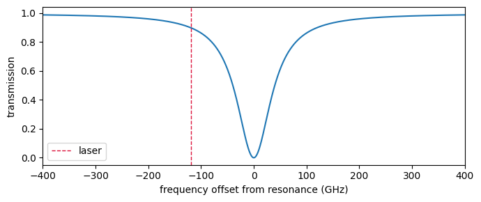
The analytic all-pass transmission is used throughout this example as a reference curve: with round-trip amplitude \(a\), coupler through coefficient \(t\), and round-trip phase \(\phi = 2\pi (f - f_\mathrm{res}) / \mathrm{FSR}\),

\[T(\phi) = \frac{a^2 - 2 a t \cos\phi + t^2}{1 - 2 a t \cos\phi + (a t)^2},\]

and the heater enters through \(f_\mathrm{res}(V) = f_\mathrm{res,0} - V \, df/dV\).

The next cell instantiates the components shared by every circuit: the laser, the monitor photodiode (10 mW and a 1000 V/A transimpedance make 10 V at full transmission), the thermal RC filter standing in for the heater’s thermal mass, the adders, and a matched termination. Parametric components with identical arguments are cached, so reusing these instances is the natural way to build many circuits around one device.

# detection chain and thermal plant, shared by all three loops
p_in = 10e-3  # laser power (W)
gain = 1e3  # transimpedance (V/A)
v_full = gain * p_in  # detected voltage at full transmission (V)
f_th = 30e6  # compressed heater thermal pole (Hz)
tau_th = 1 / (2 * np.pi * f_th)  # thermal time constant (5.3 ns here)
v_max = 5.0  # heater drive rail (V)

# one instance of each shared block, referenced by every circuit below
laser = pfa.cw_laser(power=p_in, frequency=f_laser)
pd = pfa.photodiode(responsivity=1.0, gain=gain, seed=1)  # seed fixes the shot noise
rc_thermal = pfa.filter(family="rc", f_cutoff=f_th, order=1)  # heater thermal mass
summer = pfa.adder()  # plain unit-weight adder, reused wherever signals merge
err_adder = pfa.adder(weight0=1.0, weight1=-1.0)  # error = (input 0) - (input 1)
term = pfa.electrical_termination()  # matched load for deliberately unused inputs


def allpass_t(f_res):
    # analytic all-pass transmission at the laser frequency (reference curves)
    phi = 2 * np.pi * (f_laser - f_res) / fsr  # round-trip phase offset
    a = 10 ** (-loss_db_um * length / 20)  # round-trip amplitude
    num = a**2 - 2 * a * t_c * np.cos(phi) + t_c**2
    den = 1 - 2 * a * t_c * np.cos(phi) + (a * t_c) ** 2
    return num / den


def t_static(v):
    # reference transmission as a function of heater voltage
    return allpass_t(f_res0 - df_dv * np.asarray(v, dtype=float))

Closing a Feedback Loop in the Time Domain

Two practical points about building the loop circuits:

• A feedback cycle cannot be expressed by geometric port matching, since connect moves the reference being connected. The circuits below are therefore described as netlists and built with component_from_netlist, using "virtual connections", logical links that ignore port positions. Each instance still receives its own origin: abstract components all sit near the origin, and coincident ports of unspread references would be joined geometrically before the virtual connections are considered.

• Slow externally computed drives, the heater staircases and the thermal disturbances below, are injected through exposed ports with a TimeSeries keyed by the port name, and exposed ports also return their outgoing signal, so a detector output can simply be exposed instead of monitored. Periodic drives, the data pattern and the dither tone, come from signal_source instances inside the circuits; internal pattern sources are generated fresh by each stepper run, so they suit the single-run steppers used throughout this example (a stepper must be reset before it is reused).

Flank Locking a Passive Ring

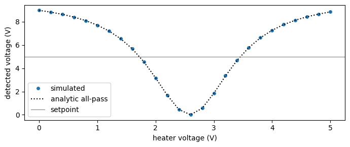
The plant is characterized first: laser through the ring into the photodiode, with the heater port exposed for a voltage staircase and the photodiode output exposed as the circuit output.

Two design numbers come out of the static curve:

• the plant slope \(dV_\mathrm{pd}/dV_h\) at the setpoint converts heater voltage to detected voltage and sets the loop gain;

• the integral gain \(k_i\) is chosen for a crossover at one third of the thermal pole, \(k_i \, \lvert dV_\mathrm{pd}/dV_h \rvert = 2\pi f_\mathrm{th}/3\), which leaves about 70 degrees of phase margin.

# characterization circuit: laser -> ring -> photodiode; the heater drive is
# injected at 'vh' and the detected voltage comes back at the exposed 'pd' port;
# origins spread the references so no default port positions coincide
char1 = pf.component_from_netlist({
    "name": "static response",
    "instances": {
        "laser": laser,
        "ring": {"component": ring, "origin": (20, 0)},
        "pd": {"component": pd, "origin": (40, 0)},
    },
    "virtual connections": [
        (("laser", "P0"), ("ring", "P0")),  # laser into the bus
        (("ring", "P1"), ("pd", "P0")),  # through port onto the photodiode
    ],
    "ports": [("ring", "E0", "vh"), ("pd", "E0", "pd")],
    "models": [(pf.CircuitModel(), "Circuit")],
})

ts = char1.setup_time_stepper(time_step=dt, carrier_frequency=f_laser,
                              show_progress=False)

# voltage staircase in ONE run: 26 plateaus of 300 ps (photon lifetime is 4 ps),
# encoded directly in the injected drive array
v_grid1 = np.linspace(0, v_max, 26)
plateau = 3000  # steps per plateau
vh_drive = np.repeat(v_grid1, plateau)  # staircase waveform (V)
out = ts.step(inputs=pf.TimeSeries({"vh@0": vh_drive / sq}, dt),
              show_progress=False)

# outgoing signal at the exposed photodiode port, converted to volts
pd_v = np.real(out["pd@0"]) * sq
# per-plateau detected voltage: average the settled last third of each plateau
v_pd_static = pd_v.reshape(len(v_grid1), plateau)[:, -plateau // 3 :].mean(axis=1)

# operating point: FIRST downward crossing of half transmission (the near flank,
# where transmission falls as heater voltage rises)
t_set = 0.5
v_set1 = v_full * t_set  # setpoint (V)
i_dip = np.argmin(v_pd_static)  # resonance crossing the laser
i_cross = np.argmax(v_pd_static[: i_dip + 1] < v_set1)
slope1 = np.gradient(v_pd_static, v_grid1)[i_cross]  # plant slope (V per V)

# integral gain for a crossover at one third of the thermal pole
k_i1 = (2 * np.pi * f_th / 3) / abs(slope1)
print(f"plant slope {slope1:.2f} V/V at the setpoint, k_i = {k_i1:.3e} 1/s")

fig, ax = plt.subplots(figsize=(7, 3), tight_layout=True)
ax.plot(v_grid1, v_pd_static, "o", ms=4, label="simulated")
ax.plot(v_grid1, v_full * t_static(v_grid1), "k:", label="analytic all-pass")
ax.axhline(v_set1, color="gray", lw=0.8, label="setpoint")
ax.set_xlabel("heater voltage (V)")
ax.set_ylabel("detected voltage (V)")
_ = ax.legend()

plant slope -6.25 V/V at the setpoint, k_i = 1.005e+07 1/s

The closed loop adds the error adder against a DC setpoint (a signal_source with zero amplitude and a constant offset), the integrator, a summing adder with an exposed port for injecting a thermal disturbance, and the thermal RC filter. On the near flank a positive error, too much light, correctly asks for more heat. The integrator limits are the heater rails, 0 to 5 V: anti-windup with a physical meaning, since the drive cannot be negative, accumulation stops at the rails instead of winding up. The integrator’s reset input stays unused here and receives the matched termination.

The circuit has no exposed optical ports at all: the loop is observed through monitors.

setpoint1 = pfa.signal_source(amplitude=0.0, offset=v_set1 / sq)  # DC setpoint
integ1 = pfa.integrator(scale=k_i1, limits=(0.0, v_max / sq))  # limits = heater rails

flank = pf.component_from_netlist({
    "name": "flank lock",
    "instances": {
        "laser": laser,
        "ring": {"component": ring, "origin": (20, 0)},
        "pd": {"component": pd, "origin": (40, 0)},
        "error": {"component": err_adder, "origin": (60, 0)},
        "setpoint": {"component": setpoint1, "origin": (80, 0)},
        "controller": {"component": integ1, "origin": (100, 0)},
        "sum": {"component": summer, "origin": (120, 0)},
        "thermal": {"component": rc_thermal, "origin": (140, 0)},
        "term": {"component": term, "origin": (160, 0)},
    },
    "virtual connections": [
        (("laser", "P0"), ("ring", "P0")),  # optical path
        (("ring", "P1"), ("pd", "P0")),
        (("pd", "E0"), ("error", "E0")),  # error = V_pd - V_set
        (("setpoint", "E0"), ("error", "E1")),
        (("error", "E2"), ("controller", "E0")),  # integral controller
        (("term", "E0"), ("controller", "E1")),  # unused reset input, terminated
        (("controller", "E2"), ("sum", "E0")),  # controller + disturbance
        (("sum", "E2"), ("thermal", "E0")),  # through the heater thermal mass
        (("thermal", "E1"), ("ring", "E0")),  # closing the loop on the heater
    ],
    "ports": [("sum", "E1", "dist")],  # thermal disturbance injected here
    "models": [(pf.CircuitModel(), "Circuit")],
})
viewer(flank)

The run covers lock acquisition from a cold start and a 0.8 V step on the disturbance port at 200 ns, the heater-referred equivalent of a sudden 4.4 K ambient shift. For comparison, the same loop is integrated as a two-state ordinary differential equation, integrator state \(V_i\) and filtered heater voltage \(V_h\), using the measured static curve as the plant:

\[\dot V_i = k_i \left( V_\mathrm{pd}(V_h) - V_\mathrm{set} \right), \qquad \dot V_h = 2 \pi f_\mathrm{th} \left( V_i + V_\mathrm{dist} - V_h \right).\]

# references follow the netlist instance order: 2 = photodiode, 5 = controller
ts = flank.setup_time_stepper(
    time_step=dt, carrier_frequency=f_laser,
    time_stepper_kwargs={"monitors": {"pd": flank.references[2]["E0"],
                                      "ctrl": flank.references[5]["E2"]}},
    show_progress=False,
)

# one 350 ns run; the disturbance steps from 0 to 0.8 V at 200 ns
t_total1, t_dist1, v_dist1 = 350e-9, 200e-9, 0.8
n1 = int(round(t_total1 / dt))
t1 = np.arange(n1) * dt
dist = np.where(t1 >= t_dist1, v_dist1, 0.0)  # disturbance waveform (V)
out = ts.step(inputs=pf.TimeSeries({"dist@0": dist / sq}, dt), show_progress=False)

# monitor traces in volts (the signal leaves each block on the '+' direction),
# block-averaged to a 10 ps grid for plotting
block = 100
pd_tr = (np.real(out["pd@0+"]) * sq).reshape(-1, block).mean(axis=1)
ctrl_tr = (np.real(out["ctrl@0+"]) * sq).reshape(-1, block).mean(axis=1)
t_dec = (np.arange(len(pd_tr)) + 0.5) * block * dt

# two-state ODE of the same loop, on the measured static curve
pd_of_v = lambda v: np.interp(v, v_grid1, v_pd_static)


def rhs1(t, y):
    v_int, v_h = y
    dv_int = k_i1 * (pd_of_v(v_h) - v_set1)  # integral of the error
    if (v_int >= v_max and dv_int > 0) or (v_int <= 0 and dv_int < 0):
        dv_int = 0.0  # anti-windup clamp, as in the integrator limits
    # first-order thermal lag toward controller output + disturbance
    dv_h = 2 * np.pi * f_th * ((v_int + (v_dist1 if t >= t_dist1 else 0.0)) - v_h)
    return [dv_int, dv_h]


sol = solve_ivp(rhs1, (0, t_total1), [0.0, 0.0], t_eval=t_dec, rtol=1e-9,
                atol=1e-12, max_step=1e-9)

fig, axes = plt.subplots(1, 2, figsize=(10, 3.2), tight_layout=True)
axes[0].plot(t_dec * 1e9, pd_tr, lw=0.8, label="circuit")
axes[0].plot(t_dec * 1e9, pd_of_v(sol.y[1]), "k:", label="ODE")
axes[0].axhline(v_set1, color="gray", lw=0.8)
axes[0].axvline(t_dist1 * 1e9, color="crimson", lw=0.8, ls="--")
axes[0].set_xlabel("time (ns)")
axes[0].set_ylabel("detected voltage (V)")
axes[0].set_title("lock acquisition and disturbance rejection")
axes[0].legend()
axes[1].plot(t_dec * 1e9, ctrl_tr, lw=0.8, label="circuit")
axes[1].plot(t_dec * 1e9, sol.y[0], "k:", label="ODE")
axes[1].axvline(t_dist1 * 1e9, color="crimson", lw=0.8, ls="--")
axes[1].set_xlabel("time (ns)")
axes[1].set_ylabel("integrator output (V)")
axes[1].set_title("controller state")
_ = axes[1].legend()

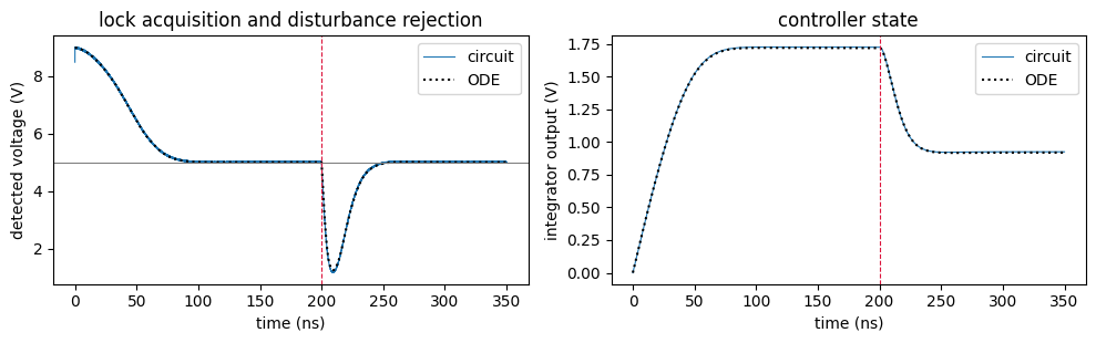
The loop settles onto the setpoint in under 100 ns, and after the disturbance step the integrator absorbs exactly the injected 0.8 V, returning the transmission to the setpoint. The photodiode shot noise, visible as fuzz on the detected voltage, is averaged away by the integrator. The circuit follows the two-state model through the whole trajectory, including the anti-windup behavior at the start: everything the loop does is captured by textbook control theory once the plant curve is known.

Mean-Power Locking a Microring Modulator

The same ring now carries data. A 25 Gb/s non-return-to-zero (NRZ) pseudorandom bit sequence (PRBS7) drives the ring’s electrical port together with the heater signal, and the laser sits on the flank so that the data swings the resonance across it: the ring is an on-off-keyed (OOK) microring modulator.

Locking a live modulator cannot use the instantaneous photodiode voltage, which now carries the data. The scheme of Padmaraju et al. [1] uses the fact that the average of a balanced bit stream is constant: the mean detected power still maps detuning one-to-one, so an RC low-pass placed after the photodiode recovers a data-independent error signal, and the same integral controller locks it.

The bit pattern comes from a signal_source with a trapezoid waveform and a built-in PRBS7 generator; a monitor on the source records the transmitted waveform, which the eye analysis below uses to tell ones from zeros. Note the recommended NRZ pulse width of \(1 + 0.5\,(\mathrm{rise} + \mathrm{fall})\) bit periods: it keeps runs of equal bits flat, at the price of widening every pulse, so the time-averaged ones density of the drive is a little higher than the 64/127 of the underlying bit sequence. The measured duty is used wherever the ones density matters.

bit_rate = 25e9
ui = int(round(1 / bit_rate / dt))  # samples per bit (400)
pattern = 127 * ui  # PRBS7 period in samples
v_pp = 0.9  # data swing on the ring port (V)

# NRZ PRBS7 pattern generator: 0 to v_pp swing, edges of 0.3 bit periods
data_src = pfa.signal_source(
    frequency=bit_rate, amplitude=v_pp / sq, waveform="trapezoid",
    rise=0.3, fall=0.3, width=1.3, prbs=7, seed=0,
)

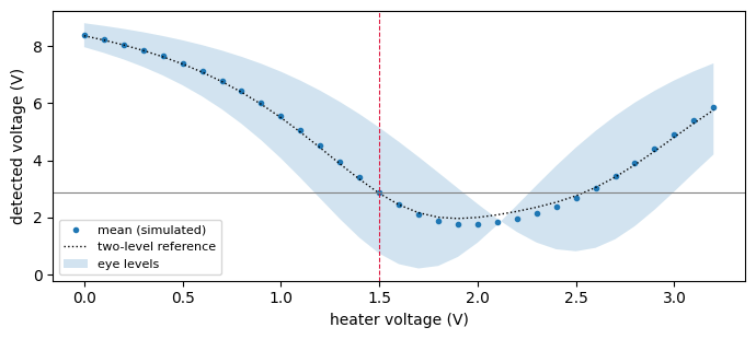
The modulated plant is characterized like the passive one, a heater staircase, but with the data running.

At each heater voltage the mean detected voltage gives the error-signal curve the loop will see, and sampling the detected signal at the pulse centers, grouped by the transmitted bit, gives the eye levels. The sampling phase is measured from the recorded drive itself, since the pulse-width convention shifts the pulse centers off the nominal bit grid. The mean of the two static bit levels, weighted by the measured ones density, is plotted for reference.

The operating point \(V^*\) is the heater voltage that maximizes the eye amplitude among points with a usable negative mean-power slope, and the setpoint is simply the measured mean there.

# characterization circuit: as before, plus an adder merging heater and data
# into the ring's single electrical port
char2 = pf.component_from_netlist({
    "name": "modulated response",
    "instances": {
        "laser": laser,
        "ring": {"component": ring, "origin": (20, 0)},
        "pd": {"component": pd, "origin": (40, 0)},
        "drive": {"component": summer, "origin": (60, 0)},
        "data": {"component": data_src, "origin": (80, 0)},
    },
    "virtual connections": [
        (("laser", "P0"), ("ring", "P0")),
        (("ring", "P1"), ("pd", "P0")),
        (("data", "E0"), ("drive", "E1")),  # data onto the drive adder
        (("drive", "E2"), ("ring", "E0")),  # heater + data onto the ring
    ],
    "ports": [("drive", "E0", "vh"), ("pd", "E0", "pd")],
    "models": [(pf.CircuitModel(), "Circuit")],
})
# the data source output is monitored to know the transmitted bits (reference 4)
ts = char2.setup_time_stepper(
    time_step=dt, carrier_frequency=f_laser,
    time_stepper_kwargs={"monitors": {"data": char2.references[4]["E0"]}},
    show_progress=False,
)


def rx_filter(x):
    # zero-phase 4th-order Bessel at 0.75 x bit rate, the display receiver
    sos = signal.bessel(4, 0.75 * bit_rate, fs=1 / dt, output="sos")
    return signal.sosfiltfilt(sos, x)


def bit_levels(pd_raw, data_raw, skip_bits=2):
    # detected voltage at pulse centers, split by the transmitted bit, which is
    # read off the recorded data waveform (both traces span the same steps);
    # bit_phase, measured below, aligns the sampling with the pulse centers
    v = rx_filter(pd_raw)
    centers = np.arange(skip_bits * ui + bit_phase, len(v), ui)
    ones = data_raw[centers] > 0.45 * v_pp  # threshold the drive at mid-swing
    return v[centers][~ones], v[centers][ones]  # levels of 0s, levels of 1s


# staircase with the data running, again in one run: per plateau, 1 pattern
# period of settling followed by 2 recorded periods (integer bit counts keep
# the pattern phase aligned with the plateau boundaries)
v_grid2 = np.arange(0, 3.21, 0.1)
settle, record = pattern, 2 * pattern
span = settle + record  # steps per plateau
out = ts.step(
    inputs=pf.TimeSeries({"vh@0": np.repeat(v_grid2, span) / sq}, dt),
    show_progress=False,
)
pd_v = np.real(out["pd@0"]) * sq  # exposed photodiode output (V)
data_v = np.real(out["data@0+"]) * sq  # transmitted NRZ waveform (V)

# measured ones density of the drive (integer pattern count makes it exact)
duty = data_v.mean() / v_pp
print(f"measured drive duty {duty:.3f} (bit density 64/127 = {64 / 127:.3f})")

# sampling phase: the width convention shifts the pulse centers, so sample in the
# MIDDLE of the flat tops; the worst-case distance from mid-swing over all bits
# scores each phase, and a circular half-bit window centers the pick in the
# flat region instead of at its edge
probe = data_v[: 10 * pattern].reshape(-1, ui)  # one column per phase offset
scores = np.abs(probe - 0.5 * v_pp).min(axis=0)  # worst-case flatness per phase
win = np.real(np.fft.ifft(np.fft.fft(scores) * np.fft.fft(np.ones(ui // 2), ui)))
bit_phase = int((np.argmax(win) - ui // 4) % ui)  # window end minus half window
print(f"pulse centers at {bit_phase} samples past the nominal bit boundary")

# slice out the recorded part of each plateau, for both traces
sl = [slice(i * span + settle, (i + 1) * span) for i in range(len(v_grid2))]
plateau_pd = [pd_v[s] for s in sl]
plateau_data = [data_v[s] for s in sl]
v_mean = np.array([p.mean() for p in plateau_pd])  # mean-power curve
levels = [bit_levels(p, d) for p, d in zip(plateau_pd, plateau_data)]
lvl0 = np.array([l0.mean() for l0, l1 in levels])  # zeros level vs heater voltage
lvl1 = np.array([l1.mean() for l0, l1 in levels])  # ones level vs heater voltage

# operating point: largest eye among points with a usable negative mean slope
eye_amp = np.abs(lvl1 - lvl0)
mean_slope = np.gradient(v_mean, v_grid2)
usable = np.where(mean_slope < -0.5)[0]
i_star = usable[np.argmax(eye_amp[usable])]
v_star = v_grid2[i_star]  # bias the loop will have to reproduce
v_set2 = v_mean[i_star]  # setpoint = measured mean at the operating point
k_i2 = (2 * np.pi * f_th / 3) / abs(mean_slope[i_star])  # same crossover rule
print(f"operating point {v_star:.1f} V: eye amplitude {eye_amp[i_star]:.2f} V, "
      f"setpoint {v_set2:.2f} V, k_i = {k_i2:.3e} 1/s")

# reference: static two-level mean weighted by the measured duty
mean_ref = v_full * ((1 - duty) * t_static(v_grid2)
                     + duty * t_static(v_grid2 + v_pp))

fig, ax = plt.subplots(figsize=(7, 3.2), tight_layout=True)
ax.plot(v_grid2, v_mean, "o", ms=3, label="mean (simulated)")
ax.plot(v_grid2, mean_ref, "k:", lw=1, label="two-level reference")
ax.fill_between(v_grid2, lvl0, lvl1, alpha=0.2, label="eye levels")
ax.axvline(v_star, color="crimson", lw=0.8, ls="--")
ax.axhline(v_set2, color="gray", lw=0.8)
ax.set_xlabel("heater voltage (V)")
ax.set_ylabel("detected voltage (V)")
_ = ax.legend(fontsize=8)

measured drive duty 0.579 (bit density 64/127 = 0.504)
pulse centers at 319 samples past the nominal bit boundary
operating point 1.5 V: eye amplitude 4.41 V, setpoint 2.89 V, k_i = 1.325e+07 1/s

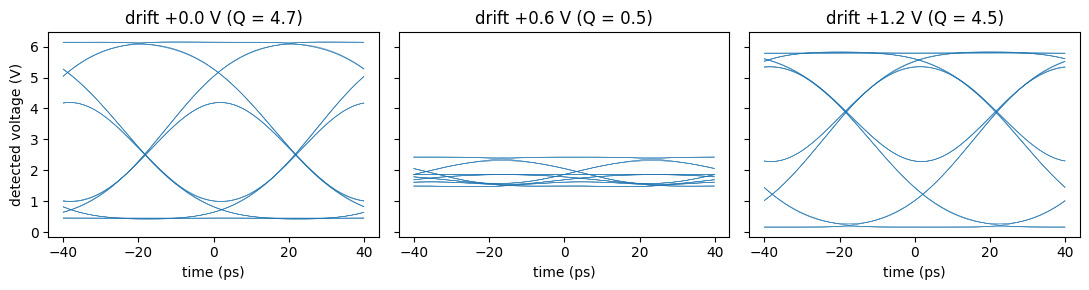
Before closing the loop, the eye diagrams below show what is at stake. At the operating point the eye is clean. A heater-referred drift of 0.6 V, about 3.3 K, collapses it. At 1.2 V of drift the resonance has crossed to the other side of the laser and an inverted eye reopens: the levels have swapped, and a receiver expecting the original polarity still fails. The eye quality factor \(Q = \lvert \mu_1 - \mu_0 \rvert / (\sigma_1 + \sigma_0)\) is printed for each case.

def eye_fold(pd_raw):
    # receiver-filtered trace folded into 2-bit segments for eye display;
    # starting at bit_phase puts pulse centers mid-plot and crossings at +-20 ps
    v = rx_filter(pd_raw)
    n_seg = (len(v) - ui) // (2 * ui)
    return v[bit_phase : bit_phase + n_seg * 2 * ui].reshape(n_seg, 2 * ui)


def eye_q(pd_raw, data_raw):
    # eye quality factor from the bit-center level statistics
    l0, l1 = bit_levels(pd_raw, data_raw)
    return abs(l0.mean() - l1.mean()) / (l0.std() + l1.std())


t_eye = (np.arange(2 * ui) - ui) * dt * 1e12  # eye time axis (ps)

fig, axes = plt.subplots(1, 3, figsize=(11, 3), tight_layout=True, sharey=True)
for ax, drift in zip(axes, [0.0, 0.6, 1.2]):
    i = i_star + int(round(drift / 0.1))  # staircase index at this drift
    q = eye_q(plateau_pd[i], plateau_data[i])
    ax.plot(t_eye, eye_fold(plateau_pd[i]).T, color="tab:blue", lw=0.3, alpha=0.25)
    ax.set_title(f"drift +{drift:.1f} V (Q = {q:.1f})")
    ax.set_xlabel("time (ps)")
_ = axes[0].set_ylabel("detected voltage (V)")
q_ref = eye_q(plateau_pd[i_star], plateau_data[i_star])

The closed-loop circuit adds the mean-power extraction filter, an RC low-pass at 60 MHz: fast enough to follow the loop dynamics, slow enough to suppress the data and the 197 MHz PRBS7 pattern repetition. Its pole costs about 10 degrees of phase at the 10 MHz crossover, which the design absorbs. Everything else is the flank-lock loop, with a second adder merging the data into the heater drive.

f_pd = 60e6  # mean-power extraction pole (Hz)
pd_filter = pfa.filter(family="rc", f_cutoff=f_pd, order=1)
setpoint2 = pfa.signal_source(amplitude=0.0, offset=v_set2 / sq)
integ2 = pfa.integrator(scale=k_i2, limits=(0.0, v_max / sq))

mrm = pf.component_from_netlist({
    "name": "modulator lock",
    "instances": {
        "laser": laser,
        "ring": {"component": ring, "origin": (20, 0)},
        "pd": {"component": pd, "origin": (40, 0)},
        "mean": {"component": pd_filter, "origin": (60, 0)},
        "error": {"component": err_adder, "origin": (80, 0)},
        "setpoint": {"component": setpoint2, "origin": (100, 0)},
        "controller": {"component": integ2, "origin": (120, 0)},
        "sum": {"component": summer, "origin": (140, 0)},
        "thermal": {"component": rc_thermal, "origin": (160, 0)},
        "drive": {"component": summer, "origin": (180, 0)},
        "data": {"component": data_src, "origin": (200, 0)},
        "term": {"component": term, "origin": (220, 0)},
    },
    "virtual connections": [
        (("laser", "P0"), ("ring", "P0")),  # optical path
        (("ring", "P1"), ("pd", "P0")),
        (("pd", "E0"), ("mean", "E0")),  # mean-power extraction
        (("mean", "E1"), ("error", "E0")),  # error = mean - setpoint
        (("setpoint", "E0"), ("error", "E1")),
        (("error", "E2"), ("controller", "E0")),
        (("term", "E0"), ("controller", "E1")),  # unused reset input
        (("controller", "E2"), ("sum", "E0")),  # controller + disturbance
        (("sum", "E2"), ("thermal", "E0")),  # heater thermal mass
        (("thermal", "E1"), ("drive", "E0")),  # slow heater + fast data
        (("data", "E0"), ("drive", "E1")),
        (("drive", "E2"), ("ring", "E0")),
    ],
    "ports": [("sum", "E1", "dist")],
    "models": [(pf.CircuitModel(), "Circuit")],
})
viewer(mrm)

The disturbance is now a 2 MHz sinusoid of 0.6 V amplitude, a compressed stand-in for kilohertz-scale ambient fluctuations, switched on at 300 ns after the loop has locked. The same disturbance is then replayed open-loop, holding the heater at the static operating point, for comparison.

t_total2, t_on2 = 900e-9, 300e-9
f_dist, a_dist = 2e6, 0.6  # disturbance frequency (Hz) and amplitude (V)
n2 = int(round(t_total2 / dt))
t2 = np.arange(n2) * dt

# closed loop: lock for 300 ns, then ride out the disturbance; references follow
# the netlist order: 2 = photodiode, 3 = mean-power filter, 10 = data source
ts = mrm.setup_time_stepper(
    time_step=dt, carrier_frequency=f_laser,
    time_stepper_kwargs={"monitors": {"pd": mrm.references[2]["E0"],
                                      "vf": mrm.references[3]["E1"],
                                      "data": mrm.references[10]["E0"]}},
    show_progress=False,
)
dist = np.where(t2 >= t_on2, a_dist * np.sin(2 * np.pi * f_dist * (t2 - t_on2)), 0.0)
out = ts.step(inputs=pf.TimeSeries({"dist@0": dist / sq}, dt), show_progress=False)
pd_c = np.real(out["pd@0+"]) * sq  # full-rate photodiode trace (for the eye)
data_c = np.real(out["data@0+"]) * sq  # transmitted bits (for the eye)
vf_c = (np.real(out["vf@0+"]) * sq).reshape(-1, block).mean(axis=1)  # mean power
t_dec2 = (np.arange(len(vf_c)) + 0.5) * block * dt

# open loop: static heater at the operating point, same disturbance from 100 ns
ts = char2.setup_time_stepper(
    time_step=dt, carrier_frequency=f_laser,
    time_stepper_kwargs={"monitors": {"data": char2.references[4]["E0"]}},
    show_progress=False,
)
t_open, t_on_o = 700e-9, 100e-9
n2o = int(round(t_open / dt))
t2o = np.arange(n2o) * dt
vh_o = v_star + np.where(
    t2o >= t_on_o, a_dist * np.sin(2 * np.pi * f_dist * (t2o - t_on_o)), 0.0)
out = ts.step(inputs=pf.TimeSeries({"vh@0": vh_o / sq}, dt), show_progress=False)
pd_o = np.real(out["pd@0"]) * sq
data_o = np.real(out["data@0+"]) * sq
pd_o_dec = pd_o.reshape(-1, block).mean(axis=1)
t_dec_o = (np.arange(len(pd_o_dec)) + 0.5) * block * dt

# a boxcar over one PRBS period removes the pattern-repetition ripple from the
# mean-power traces before comparing them
box = pattern // block  # decimated samples per PRBS period
pbox = lambda x: np.convolve(x, np.ones(box) / box, mode="valid")
t_b2 = t_dec2[box - 1 :] - (box - 1) * block * dt / 2
t_bo = t_dec_o[box - 1 :] - (box - 1) * block * dt / 2


def tone_amp(t, x):
    # least-squares amplitude of the disturbance tone (plus a DC term)
    basis = np.stack([np.sin(2 * np.pi * f_dist * t), np.cos(2 * np.pi * f_dist * t),
                      np.ones_like(t)], axis=1)
    c = np.linalg.lstsq(basis, x, rcond=None)[0]
    return np.hypot(c[0], c[1])


# residual mean-power wobble at the disturbance frequency, closed vs open
amp_c = tone_amp(t_b2[t_b2 > 400e-9], pbox(vf_c)[t_b2 > 400e-9])
amp_o = tone_amp(t_bo[t_bo > 200e-9], pbox(pd_o_dec)[t_bo > 200e-9])
print(f"mean-power wobble {amp_o:.2f} V open loop, {amp_c:.2f} V closed loop: "
      f"suppressed {amp_o / amp_c:.1f}x")

fig, ax = plt.subplots(figsize=(9, 3.2), tight_layout=True)
ax.plot(t_b2 * 1e9, pbox(vf_c), lw=0.8, label="closed loop")
ax.plot(t_bo * 1e9, pbox(pd_o_dec), lw=0.8, color="tab:orange",
        label="open loop, same disturbance")
ax.axhline(v_set2, color="gray", lw=0.8)
ax.axvline(t_on2 * 1e9, color="crimson", lw=0.8, ls="--")
ax.set_xlabel("time (ns)")
ax.set_ylabel("mean detected voltage (V)")
_ = ax.legend(fontsize=8)

mean-power wobble 2.26 V open loop, 0.57 V closed loop: suppressed 4.0x

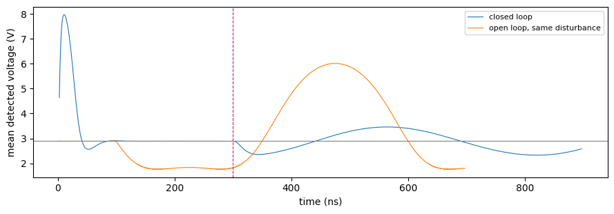
The loop suppresses the mean-power wobble by a factor of about four. The small-signal expectation is \(\lvert 1 + L(j\omega) \rvert\) with the loop transmission \(L = k_i \, \lvert dV_\mathrm{pd}/dV_h \rvert \, H_\mathrm{th} H_\mathrm{pd} / (j\omega)\), about 5 at 2 MHz; the measured ratio is a little lower because the 0.6 V disturbance is not small, it explores the curvature of the plant around the operating point.

The eye diagrams tell the same story at the data layer: with the loop closed, the eye stays open through the disturbance, while the open-loop eye is destroyed. The eyes are built from the final 300 ns of each run, so they average over the disturbance phases.

keep_c = int(round(600e-9 / dt))  # closed-loop eye: the final 300 ns
keep_o = int(round(400e-9 / dt))  # open-loop eye: the final 300 ns

fig, axes = plt.subplots(1, 3, figsize=(11, 3), tight_layout=True, sharey=True)
cases = [
    (plateau_pd[i_star], plateau_data[i_star], "locked, no disturbance",
     "tab:blue", 1),
    (pd_c[keep_c:], data_c[keep_c:], "closed loop + disturbance", "tab:green", 3),
    (pd_o[keep_o:], data_o[keep_o:], "open loop + disturbance", "tab:orange", 3),
]
for ax, (trace, bits, title, color, stride) in zip(axes, cases):
    q = eye_q(trace, bits)
    ax.plot(t_eye, eye_fold(trace)[::stride].T, color=color, lw=0.3, alpha=0.15)
    ax.set_title(f"{title} (Q = {q:.1f})")
    ax.set_xlabel("time (ps)")
_ = axes[0].set_ylabel("detected voltage (V)")

Dither Locking to the Resonance Extremum

Both loops so far lock to a flank, which fails exactly where many applications need to operate: at the transmission extremum, the mean-power error signal has zero slope, so a flank lock parked there has no gain and cannot even tell which way the resonance drifted. The standard answer, demonstrated for microrings by Padmaraju et al. [2], is a dither lock, the optical version of lock-in detection:

• a small dither tone rides on the heater drive (here 200 MHz at 0.1 V, a 4.6 GHz resonance wiggle, small compared to the 79 GHz linewidth);

• the photodiode signal is multiplied by a reference copy of the dither (multiplier, an ideal mixer) and low-pass filtered;

• the filtered product is proportional to the transmission derivative \(dT/dV\): it forms a dispersive discriminant, an S-curve, that crosses zero exactly at the extremum with a steep slope, and its sign tells the controller which way to steer.

No setpoint source is needed: the integrator simply nulls the discriminant. The dither and the demodulation reference are two sine signal_source instances at the same frequency; their phases are deterministic and equal, and a common phase offset would cancel in the demodulated product anyway. With the mixer scale set to \(-\sqrt{z_0}\), the mixer output in volts is \(-V_\mathrm{pd} V_\mathrm{lo}\), and the resulting error has the sign that makes more heat the correct response left of the extremum.

The discriminant is first measured open-loop with the heater staircase. The reference curve is the dither-cycle average of the analytic transmission, \(-\overline{v_\mathrm{full} \, T(V + A_d \sin\theta) \sin\theta}\). Note the first plateau: the lock-in filter starts from zero state, so the first point gets a longer settle than the staircase steps that follow, which inherit an almost-settled state.

f_d, a_d, a_lo = 200e6, 0.1, 1.0  # dither frequency, amplitude, reference amplitude
f_lp = 20e6  # lock-in low-pass (Hz)
dith_period = int(round(1 / f_d / dt))  # dither period in samples

mixer = pfa.multiplier(scale=-sq)  # output in volts: -v_pd * v_lo (see text)
lock_filter = pfa.filter(family="rc", f_cutoff=f_lp, order=1)
dither_src = pfa.signal_source(waveform="sine", frequency=f_d, amplitude=a_d / sq)
lo_src = pfa.signal_source(waveform="sine", frequency=f_d, amplitude=a_lo / sq)

char3 = pf.component_from_netlist({
    "name": "discriminant response",
    "instances": {
        "laser": laser,
        "ring": {"component": ring, "origin": (20, 0)},
        "pd": {"component": pd, "origin": (40, 0)},
        "mixer": {"component": mixer, "origin": (60, 0)},
        "lockin": {"component": lock_filter, "origin": (80, 0)},
        "lo": {"component": lo_src, "origin": (100, 0)},
        "dither": {"component": dither_src, "origin": (120, 0)},
        "drive": {"component": summer, "origin": (140, 0)},
    },
    "virtual connections": [
        (("laser", "P0"), ("ring", "P0")),
        (("ring", "P1"), ("pd", "P0")),
        (("pd", "E0"), ("mixer", "E0")),  # photodiode times dither reference
        (("lo", "E0"), ("mixer", "E1")),
        (("mixer", "E2"), ("lockin", "E0")),  # low-pass keeps the DC product
        (("dither", "E0"), ("drive", "E1")),  # dither rides on the heater
        (("drive", "E2"), ("ring", "E0")),
    ],
    "ports": [("drive", "E0", "vh"), ("lockin", "E1", "err")],
    "models": [(pf.CircuitModel(), "Circuit")],
})
ts = char3.setup_time_stepper(time_step=dt, carrier_frequency=f_laser,
                              show_progress=False)

# staircase in one run; per plateau: settle (10 dither periods for the first,
# 3 after that) + 2 recorded periods
v_grid3 = np.arange(0.0, 3.21, 0.1)
record3 = 2 * dith_period
spans = [(10 if j == 0 else 3) * dith_period + record3
         for j in range(len(v_grid3))]
offsets = np.concatenate([[0], np.cumsum(spans)])  # plateau boundaries (steps)
vh3 = np.concatenate([np.full(s, v) for s, v in zip(spans, v_grid3)])  # staircase
out = ts.step(inputs=pf.TimeSeries({"vh@0": vh3 / sq}, dt), show_progress=False)
err_v = np.real(out["err@0"]) * sq  # exposed lock-in output (V)

# per plateau: average the recorded (integer) dither periods at the end
err_meas = np.array([err_v[offsets[j + 1] - record3 : offsets[j + 1]].mean()
                     for j in range(len(v_grid3))])

# reference: dither-cycle average of the analytic transmission times the reference
theta = np.linspace(0, 2 * np.pi, 401)[:-1]
err_ref = np.array([
    -np.mean(v_full * t_static(v + a_d * np.sin(theta)) * a_lo * np.sin(theta))
    for v in v_grid3])

# lock point and loop gain from the measured discriminant
v_res = 1.5 * fwhm / df_dv  # heater voltage aligning the resonance with the laser
i_res3 = np.argmin(np.abs(v_grid3 - v_res))
slope3 = np.gradient(err_meas, v_grid3)[i_res3]  # discriminant slope at the zero
k_i3 = (2 * np.pi * f_lp / 3.3) / abs(slope3)  # crossover below both loop poles
print(f"discriminant slope {slope3:.2f} V/V at the extremum, k_i = {k_i3:.3e} 1/s")

fig, ax = plt.subplots(figsize=(7, 3.4), tight_layout=True)
ax.plot(v_grid3, err_meas, "o", ms=4, label="lock-in output")
ax.plot(v_grid3, err_ref, "k:", label="dither-averaged reference")
ax.axhline(0, color="gray", lw=0.8)
ax.axvline(v_res, color="crimson", lw=0.8, ls="--", label="resonance")
ax2 = ax.twinx()
ax2.plot(v_grid3, v_full * t_static(v_grid3), color="tab:orange", lw=1, alpha=0.6)
ax2.set_ylabel("mean detected voltage (V)", color="tab:orange")
ax.set_xlabel("heater voltage (V)")
ax.set_ylabel("error signal (V)")
ax.set_title("the discriminant crosses zero where the flank slope vanishes")
_ = ax.legend(fontsize=8)

discriminant slope -1.30 V/V at the extremum, k_i = 2.932e+07 1/s

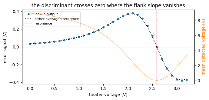
The S-curve also shows the capture range of a dither lock: the error signal has support only within about a linewidth of the resonance, so acquisition must start inside it. The integrator start_value places the loop at 2.0 V, inside the capture range but well off the extremum. After acquisition, a 0.4 V step is applied to the thermal disturbance port.

The reference model keeps the dither explicit instead of averaging it away:

\[\dot V_i = k_i V_f, \qquad \dot V_h = 2 \pi f_\mathrm{th} (V_i + V_\mathrm{dist} - V_h), \qquad \dot V_f = 2 \pi f_\mathrm{lp} \left( -v_\mathrm{full} \, T(V_h + A_d \sin \omega_d t) \, A_\mathrm{lo} \sin \omega_d t - V_f \right).\]

During acquisition the heater slews through the capture range within a few dither periods, and the demodulator output there is a transient that a dither-averaged discriminant cannot represent; keeping the \(\sin \omega_d t\) terms costs nothing and the only physics assumption left is that the cavity responds quasi-statically, well justified with a 4 ps photon lifetime against a 5 ns dither period.

v_start = 2.0  # acquisition start, inside the capture range
integ3 = pfa.integrator(scale=k_i3, start_value=v_start / sq,
                        limits=(0.0, v_max / sq))

dlock = pf.component_from_netlist({
    "name": "dither lock",
    "instances": {
        "laser": laser,
        "ring": {"component": ring, "origin": (20, 0)},
        "pd": {"component": pd, "origin": (40, 0)},
        "mixer": {"component": mixer, "origin": (60, 0)},
        "lockin": {"component": lock_filter, "origin": (80, 0)},
        "controller": {"component": integ3, "origin": (100, 0)},
        "sum": {"component": summer, "origin": (120, 0)},
        "thermal": {"component": rc_thermal, "origin": (140, 0)},
        "drive": {"component": summer, "origin": (160, 0)},
        "lo": {"component": lo_src, "origin": (180, 0)},
        "dither": {"component": dither_src, "origin": (200, 0)},
        "term": {"component": term, "origin": (220, 0)},
    },
    "virtual connections": [
        (("laser", "P0"), ("ring", "P0")),
        (("ring", "P1"), ("pd", "P0")),
        (("pd", "E0"), ("mixer", "E0")),  # lock-in detection
        (("lo", "E0"), ("mixer", "E1")),
        (("mixer", "E2"), ("lockin", "E0")),
        (("lockin", "E1"), ("controller", "E0")),  # integrator nulls the S-curve
        (("term", "E0"), ("controller", "E1")),  # unused reset input
        (("controller", "E2"), ("sum", "E0")),  # controller + disturbance
        (("sum", "E2"), ("thermal", "E0")),  # heater thermal mass
        (("thermal", "E1"), ("drive", "E0")),  # slow heater + fast dither
        (("dither", "E0"), ("drive", "E1")),
        (("drive", "E2"), ("ring", "E0")),
    ],
    "ports": [("sum", "E1", "dist")],
    "models": [(pf.CircuitModel(), "Circuit")],
})

# references follow the netlist instance order: 2 = photodiode, 5 = controller
ts = dlock.setup_time_stepper(
    time_step=dt, carrier_frequency=f_laser,
    time_stepper_kwargs={"monitors": {"pd": dlock.references[2]["E0"],
                                      "ctrl": dlock.references[5]["E2"]}},
    show_progress=False,
)

# one 700 ns run: acquisition from 2.0 V, then a 0.4 V thermal step at 350 ns
t_total3, t_step3, a_step3 = 700e-9, 350e-9, 0.4
n3 = int(round(t_total3 / dt))
t3 = np.arange(n3) * dt
out = ts.step(
    inputs=pf.TimeSeries({"dist@0": np.where(t3 >= t_step3, a_step3, 0.0) / sq},
                         dt),
    show_progress=False,
)
pd3 = (np.real(out["pd@0+"]) * sq).reshape(-1, block).mean(axis=1)
ctrl3 = (np.real(out["ctrl@0+"]) * sq).reshape(-1, block).mean(axis=1)
t_dec3 = (np.arange(len(pd3)) + 0.5) * block * dt

# explicit-dither reference model (three states, see the equations above)
w_d = 2 * np.pi * f_d


def rhs3(t, y):
    v_int, v_h, v_f = y
    s = np.sin(w_d * t)
    err = -v_full * t_static(v_h + a_d * s) * a_lo * s  # instantaneous mixer output
    dv_int = k_i3 * v_f  # the integrator input is the filtered product
    if (v_int >= v_max and dv_int > 0) or (v_int <= 0 and dv_int < 0):
        dv_int = 0.0  # anti-windup clamp
    dv_h = 2 * np.pi * f_th * ((v_int + (a_step3 if t >= t_step3 else 0.0)) - v_h)
    dv_f = 2 * np.pi * f_lp * (err - v_f)  # lock-in low-pass
    return [dv_int, dv_h, dv_f]


# max_step resolves the dither oscillation (20 points per period)
sol = solve_ivp(rhs3, (0, t_total3), [v_start, 0.0, 0.0], t_eval=t_dec3,
                rtol=1e-8, atol=1e-11, max_step=2.5e-10)
pd_ode3 = v_full * t_static(sol.y[1] + a_d * np.sin(w_d * t_dec3))

# a boxcar over one dither period removes the demodulation ripple for display
box3 = dith_period // block
pb3 = lambda x: np.convolve(x, np.ones(box3) / box3, mode="valid")
t_b3 = t_dec3[box3 - 1 :] - (box3 - 1) * block * dt / 2

lock_v = pb3(ctrl3)[(t_b3 > t_step3 - 30e-9) & (t_b3 < t_step3)].mean()
final_v = pb3(ctrl3)[t_b3 > t_total3 - 30e-9].mean()
print(f"locked at {lock_v:.3f} V; after the 0.4 V step the integrator "
      f"holds {final_v:.3f} V")

fig, axes = plt.subplots(1, 2, figsize=(10, 3.2), tight_layout=True)
axes[0].plot(t_b3 * 1e9, pb3(ctrl3), lw=0.8, label="circuit")
axes[0].plot(t_b3 * 1e9, pb3(sol.y[0]), "k:", label="explicit-dither ODE")
axes[0].axhline(v_res, color="gray", lw=0.8)
axes[0].axvline(t_step3 * 1e9, color="crimson", lw=0.8, ls="--")
axes[0].set_xlabel("time (ns)")
axes[0].set_ylabel("integrator output (V)")
axes[0].set_title("acquisition and step rejection")
axes[0].legend(fontsize=8)
axes[1].plot(t_b3 * 1e9, pb3(pd3), lw=0.8, label="circuit")
axes[1].plot(t_b3 * 1e9, pb3(pd_ode3), "k:", label="explicit-dither ODE")
axes[1].axvline(t_step3 * 1e9, color="crimson", lw=0.8, ls="--")
axes[1].set_xlabel("time (ns)")
axes[1].set_ylabel("mean detected voltage (V)")
axes[1].set_title("transmission pinned to the extremum")
_ = axes[1].legend(fontsize=8)

locked at 2.587 V; after the 0.4 V step the integrator holds 2.187 V

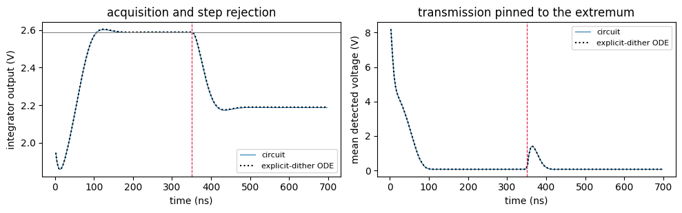
The loop pulls the ring onto the extremum, holds the transmission at its dither-limited minimum, well under 1% of the full-scale detected voltage, and after the disturbance step the integrator absorbs exactly the injected 0.4 V while the transmission returns to the minimum: the loop stays locked at the very point where the flank schemes of the previous sections have no error signal at all.

Final Remarks

• The controllers here are pure integrators, and every design number came from a measured static curve plus one crossover choice. The same blocks extend directly to proportional-integral-derivative control: a scaler for the P term and a differentiator for the D term, summed with adders.

• The heater was linearized through dn_dv. The quadratic dependence of heating power on drive voltage can be modeled with the ring’s dn_dv2 term, or with a squaring ExpressionTimeStepper block in the drive path; the loop then sees a bias-dependent plant gain.

• All timescales below the cavity linewidth were compressed to keep the runs short. To map a design to physical microsecond heaters, scale \(f_\mathrm{th}\), the filter cutoffs, the dither frequency, and the disturbance spectrum down together, and reduce the integral gains by the same factor: the loop shapes, phase margins, and suppression ratios are unchanged.

• Photodiode shot noise was present in every run and is what the residual fuzz on the detected traces shows; the loops average it. Receiver thermal noise, dark current, and finite photodiode bandwidth are available on the photodiode model for noise budget studies.