Electrical Amplifier

Between the signal source and the modulator sits a driver, and between the photodiode and the decision circuit an amplifier chain: real electrical amplifiers add gain, but also band-limit, distort, and add noise. The ElectricalAmplifierTimeStepper models a broadband amplifier or modulator driver as a two-port block that processes the signal through the classic chain of RF impairments:

1. Linear gain and a first-order low-pass for the bandwidth (gain, f_3dB),

2. soft-knee 1 dB compression (compression_power),

3. cubic third-order nonlinearity (ip3),

4. smooth output saturation (saturation_power),

5. additive noise derived from the noise figure (noise_figure), plus port reflections r0 and r1.

Electrical amplitudes are \(V / \sqrt{Z_0}\), so a sine of peak voltage \(V_m\) carries the average power \(P = V_m^2 / (2 Z_0)\), the quantity behind all the dBm-valued arguments. This guide measures the frequency response, traces gain compression and saturation, runs the classic two-tone intermodulation test, and checks the output noise floor.

Setup

import matplotlib.pyplot as plt
import numpy as np
import photonforge as pf
import photonforge.abstract as pfa

viewer = pf.live_viewer.LiveViewer()

LiveViewer started at http://localhost:62998

tech = pf.basic_technology()
pf.config.default_technology = tech

f0 = pf.C_0 / 1.55
z0 = 50.0
time_step = 1e-12
kb_t0 = 1.380649e-23 * 290


def dbm(power):
    return 10 * np.log10(power / 1e-3)

Gain and Bandwidth

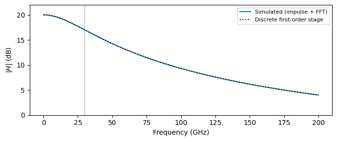
The abstract electrical_amplifier amplifies from E0 to E1. Like any component, it can be simulated on its own, without wrapping it in a circuit: setup_time_stepper runs directly on the component, and input signals are injected as a TimeSeries keyed by its own port names. Since the block is linear at small signals, a single injected impulse and an FFT measure the whole frequency response. The bandwidth limit is implemented as the exact discrete-time first-order filter

\[y[n] = \alpha y[n-1] + (1 - \alpha) \, G_a \, a_\mathrm{in} \qquad \alpha = e^{-2 \pi f_{3\mathrm{dB}} \Delta t}\]

whose response is drawn as the dotted reference; at frequencies well below \(1 / \Delta t\) it coincides with the familiar analog pole.

gain_db = 20
f_3db = 30e9
amplifier = pfa.electrical_amplifier(gain=gain_db, f_3dB=f_3db)
viewer(amplifier)

num_steps = 4096
time_stepper = amplifier.setup_time_stepper(
    time_step=time_step, carrier_frequency=f0, show_progress=False
)
v_in = np.zeros(num_steps)
v_in[0] = 1e-3
output = time_stepper.step(inputs=pf.TimeSeries({"E0@0": v_in}, time_step), show_progress=False)
h = np.fft.rfft(np.real(output["E1@0"])) / 1e-3
freq = np.fft.rfftfreq(num_steps, time_step)

# Exact response of the discrete-time first-order stage
alpha = np.exp(-2 * np.pi * f_3db * time_step)
h_ref = 10 ** (gain_db / 20) * (1 - alpha) / np.abs(1 - alpha * np.exp(-2j * np.pi * freq * time_step))

fig, ax = plt.subplots(figsize=(7, 3), tight_layout=True)
band = freq < 200e9
ax.plot(freq[band] / 1e9, 20 * np.log10(np.abs(h[band])), label="Simulated (impulse + FFT)")
ax.plot(freq[band] / 1e9, 20 * np.log10(h_ref[band]), "k:", label="Discrete first-order stage")
ax.axvline(f_3db / 1e9, color="k", linewidth=0.5, alpha=0.5)
ax.set(xlabel="Frequency (GHz)", ylabel="$|H|$ (dB)", ylim=(0, 22))
_ = ax.legend(fontsize=8)

Gain Compression and Saturation

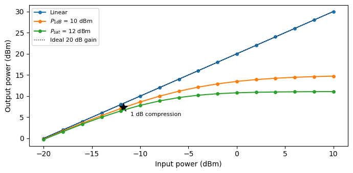
Driving harder eventually stops paying: the compression_power argument sets the output power at which the soft-knee stage has taken 1 dB off the linear gain, and saturation_power clamps the output amplitude entirely through a smooth tanh. Sweeping a single tone’s input power maps the \(P_\mathrm{out}\) vs \(P_\mathrm{in}\) characteristic of three devices: ideal, compressing, and saturating. The dot marks the measured 1 dB compression point of the middle device.

tone_freq = 5e9
num_steps = 20000
t = np.arange(num_steps) * time_step
settled = slice(num_steps // 2, None)

devices = {
    "Linear": pfa.electrical_amplifier(gain=gain_db),
    "$P_{1dB}$ = 10 dBm": pfa.electrical_amplifier(gain=gain_db, compression_power=10),
    "$P_{sat}$ = 12 dBm": pfa.electrical_amplifier(gain=gain_db, saturation_power=12),
}

p_in_dbm = np.linspace(-20, 10, 16)
fig, ax = plt.subplots(figsize=(7, 3.5), tight_layout=True)
for label, device in devices.items():
    p_out_dbm = []
    for p_in in p_in_dbm:
        v_peak = np.sqrt(2 * 10 ** (p_in / 10) * 1e-3)
        v_in = v_peak * np.sin(2 * np.pi * tone_freq * t)
        time_stepper = device.setup_time_stepper(
            time_step=time_step, carrier_frequency=f0, show_progress=False
        )
        v = np.real(
            time_stepper.step(inputs=pf.TimeSeries({"E0@0": v_in}, time_step), show_progress=False)["E1@0"]
        )
        # Fundamental tone amplitude by lock-in
        tone = 2 * np.abs(np.mean(v[settled] * np.exp(-2j * np.pi * tone_freq * t[settled])))
        p_out_dbm.append(dbm(tone**2 / 2))
    p_out_dbm = np.array(p_out_dbm)
    ax.plot(p_in_dbm, p_out_dbm, "o-", markersize=4, label=label)
    if "1dB" in label:
        deficit = (p_in_dbm + gain_db) - p_out_dbm
        p1db_in = np.interp(1.0, deficit, p_in_dbm)
        p1db_out = np.interp(p1db_in, p_in_dbm, p_out_dbm)
        ax.plot(p1db_in, p1db_out, "k*", markersize=12)
        ax.annotate("1 dB compression", (p1db_in, p1db_out), textcoords="offset points",
                    xytext=(10, -12), fontsize=8)

ax.plot(p_in_dbm, p_in_dbm + gain_db, "k:", linewidth=1, label="Ideal 20 dB gain")
ax.set(xlabel="Input power (dBm)", ylabel="Output power (dBm)")
_ = ax.legend(fontsize=8)

Two-Tone Intermodulation

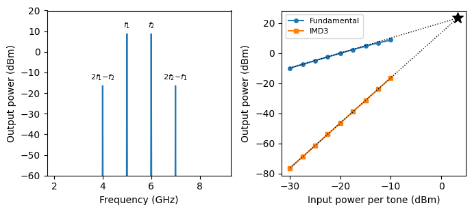
Third-order nonlinearity is invisible with a single tone in a narrow band, so it is characterized with two closely spaced tones at \(f_1\) and \(f_2\): the cubic term mixes them into intermodulation products at \(2 f_1 - f_2\) and \(2 f_2 - f_1\), right next to the signals where no filter can remove them. Their power grows with a slope of 3 on a dB scale while the fundamentals grow with slope 1, and extrapolating both lines to their crossing locates the third-order intercept point, the standard single-number linearity metric.

We inject the two-tone waveform directly as a TimeSeries and read both products from the output spectrum.

f1, f2 = 5e9, 6e9
amplifier_ip3 = pfa.electrical_amplifier(gain=gain_db, ip3=25)

num_steps = 40000
t = np.arange(num_steps) * time_step
settled = slice(num_steps // 2, None)


def tone_power_dbm(v, f):
    amplitude = 2 * np.abs(np.mean(v[settled] * np.exp(-2j * np.pi * f * t[settled])))
    return dbm(amplitude**2 / 2)


p_in_sweep = np.linspace(-30, -10, 9)
p_fund = []
p_imd3 = []
for p_in in p_in_sweep:
    v_peak = np.sqrt(2 * 10 ** (p_in / 10) * 1e-3)
    v_in = v_peak * (np.sin(2 * np.pi * f1 * t) + np.sin(2 * np.pi * f2 * t))
    time_stepper = amplifier_ip3.setup_time_stepper(
        time_step=time_step, carrier_frequency=f0, show_progress=False
    )
    v = np.real(
        time_stepper.step(inputs=pf.TimeSeries({"E0@0": v_in}, time_step), show_progress=False)["E1@0"]
    )
    p_fund.append(tone_power_dbm(v, f1))
    p_imd3.append(tone_power_dbm(v, 2 * f2 - f1))
p_fund = np.array(p_fund)
p_imd3 = np.array(p_imd3)

# spectrum at the last (strongest) drive for the left panel
spectrum = 2 * np.abs(np.fft.rfft(v[settled])) / len(v[settled])
freq = np.fft.rfftfreq(len(v[settled]), time_step)

# extrapolated third-order intercept from the two slopes
oip3 = p_fund[0] + (p_fund[0] - p_imd3[0]) / 2

fig, (ax1, ax2) = plt.subplots(1, 2, figsize=(7, 3.2), tight_layout=True)
band = (freq > 2e9) & (freq < 9e9)
ax1.plot(freq[band] / 1e9, dbm(spectrum[band] ** 2 / 2))
for f, name in [(f1, "$f_1$"), (f2, "$f_2$"), (2 * f1 - f2, "$2f_1{-}f_2$"), (2 * f2 - f1, "$2f_2{-}f_1$")]:
    ax1.annotate(name, (f / 1e9, tone_power_dbm(v, f) + 3), ha="center", fontsize=8)
ax1.set(xlabel="Frequency (GHz)", ylabel="Output power (dBm)", ylim=(-60, 20))
ax2.plot(p_in_sweep, p_fund, "o-", markersize=4, label="Fundamental")
ax2.plot(p_in_sweep, p_imd3, "s-", markersize=4, label="IMD3")
x = np.linspace(-30, oip3 - gain_db, 50)
ax2.plot(x, x + gain_db, "k:", linewidth=1)
ax2.plot(x, 3 * x + (p_imd3[0] - 3 * p_in_sweep[0]), "k:", linewidth=1)
ax2.plot(oip3 - gain_db, oip3, "k*", markersize=12)
ax2.set(xlabel="Input power per tone (dBm)", ylabel="Output power (dBm)")
ax2.legend(fontsize=8)

print(f"IMD3 slope: {(p_imd3[-1] - p_imd3[0]) / (p_in_sweep[-1] - p_in_sweep[0]):.2f} dB/dB")
print(f"Extrapolated third-order intercept (output-referred): {oip3:.1f} dBm")

IMD3 slope: 3.00 dB/dB
Extrapolated third-order intercept (output-referred): 23.2 dBm

Output Noise

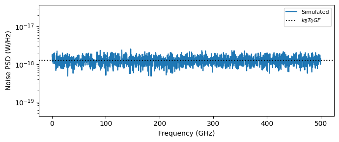
With noise_figure set, the amplifier adds white Gaussian noise at its output with the power spectral density \(S_P = k_B T_0 \, G \, F\), where \(G\) and \(F\) are the linear gain and noise factor and \(T_0 = 290\) K, the definition of noise figure for a matched input at the reference temperature. Driving the amplifier with a silent input isolates this noise, and its measured spectral density lies on the formula.

nf_db = 5
amplifier_noise = pfa.electrical_amplifier(gain=gain_db, noise_figure=nf_db, seed=0)

num_steps = 2**16
time_stepper = amplifier_noise.setup_time_stepper(
    time_step=time_step, carrier_frequency=f0, show_progress=False
)
v = np.real(
    time_stepper.step(inputs=pf.TimeSeries({"E0@0": np.zeros(num_steps)}, time_step),
                      show_progress=False)["E1@0"]
)

num_segments = 16
seg_len = num_steps // num_segments
psd = np.zeros(seg_len // 2 + 1)
for k in range(num_segments):
    seg = v[k * seg_len : (k + 1) * seg_len]
    psd += 2 * np.abs(np.fft.rfft(seg)) ** 2 * time_step / seg_len
psd /= num_segments
freq = np.fft.rfftfreq(seg_len, time_step)

s_ref = kb_t0 * 10 ** (gain_db / 10) * 10 ** (nf_db / 10)

fig, ax = plt.subplots(figsize=(7, 3), tight_layout=True)
ax.semilogy(freq[1:] / 1e9, psd[1:], label="Simulated")
ax.axhline(s_ref, color="k", linestyle=":", label="$k_B T_0 G F$")
ax.set(xlabel="Frequency (GHz)", ylabel="Noise PSD (W/Hz)", ylim=(s_ref / 30, s_ref * 30))
ax.legend(fontsize=8)

print(f"Measured output noise PSD: {psd[1:].mean():.3e} W/Hz "
      f"(k_B T_0 G F = {s_ref:.3e} W/Hz)")

Measured output noise PSD: 1.265e-18 W/Hz (k_B T_0 G F = 1.266e-18 W/Hz)

Summary

• pfa.electrical_amplifier is a two-port driver/amplifier block processing the signal through gain, a first-order bandwidth limit, soft-knee 1 dB compression, cubic third-order distortion, smooth saturation, and additive noise, with port reflections available through r0 and r1.

• A single injected impulse measures the full small-signal response; the bandwidth stage is the exact discrete-time filter given in the model documentation.

• compression_power and saturation_power (both in dBm of average sine power, \(V_m^2 / 2 Z_0\)) shape the large-signal \(P_\mathrm{out}\) vs \(P_\mathrm{in}\) characteristic.

• The two-tone test exposes the third-order nonlinearity: intermodulation products grow with slope 3, and the extrapolated intercept summarizes the linearity set by ip3.

• The output noise density follows \(k_B T_0 G F\) from noise_figure; seed makes realizations reproducible.

• Typical companions in a link: the signal_source it amplifies, the PhotodiodeTimeStepper it follows as a post-amplifier, the FilterTimeStepper for additional response shaping, and the OpticalAmplifierTimeStepper as its optical counterpart.