Laser Dynamics with External Optical Feedback

A semiconductor laser that receives a delayed reflection of its own light is a delay dynamical system. The Lang-Kobayashi model [1] describes it with the single-mode laser rate equations plus one extra term: the field emitted a round trip earlier, re-injected into the cavity with a strength \(\kappa\) and a phase \(C_p\). Depending on the feedback strength and phase, the laser emits a stable beam, oscillates at gigahertz frequencies, or becomes chaotic. The classification of these behaviors into five regimes by Tkach and Chraplyvy [2] is the reason optical isolators exist, and the reason back-reflection budgets matter in isolator-free photonic links.

This example builds a feedback laser from time-domain compact models:

• A custom TimeStepper implements a directly modulated laser that also accepts coherent optical injection at its output port. The rate equations are the same as in the built-in DMLaserTimeStepper; only the injection term is new.

• The external cavity is an ordinary circuit: a phase tuner, a waveguide, and a mirror. The delayed feedback term of the Lang-Kobayashi equations is not coded anywhere; it emerges from the circuit topology.

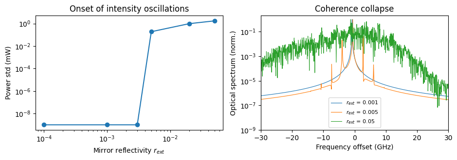
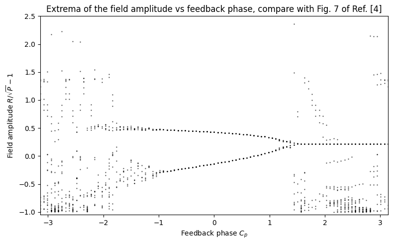
With this setup we trace the route from stable emission through relaxation-oscillation undamping to coherence collapse as the mirror reflectivity increases, and then reproduce the short-cavity bifurcation scenario reported by Heil et al. [3, 4]: sweeping the feedback phase with the intracavity tuner takes the laser from steady emission through a Hopf bifurcation and quasi-periodicity into the regular pulse package regime.

References

1. Lang, R., and Kobayashi, K. “External optical feedback effects on semiconductor injection laser properties.” IEEE Journal of Quantum Electronics 1980 16 (3), 347-355, doi: 10.1109/JQE.1980.1070479.

2. Tkach, R., and Chraplyvy, A. “Regimes of feedback effects in 1.5-um distributed feedback lasers.” Journal of Lightwave Technology 1986 4 (11), 1655-1661, doi: 10.1109/JLT.1986.1074666.

3. Heil, T., Fischer, I., Elsaesser, W., and Gavrielides, A. “Dynamics of semiconductor lasers subject to delayed optical feedback: the short cavity regime.” Physical Review Letters 2001 87 (24), 243901, doi: 10.1103/PhysRevLett.87.243901.

4. Heil, T., Fischer, I., Elsaesser, W., Krauskopf, B., Green, K., and Gavrielides, A. “Delay dynamics of semiconductor lasers with short external cavities: bifurcation scenarios and mechanisms.” Physical Review E 2003 67 (6), 066214, doi: 10.1103/PhysRevE.67.066214.

import matplotlib.pyplot as plt
import numpy as np
import photonforge as pf
import photonforge.abstract as pfa
import photonforge.typing as pft

viewer = pf.live_viewer.LiveViewer()

LiveViewer started at http://localhost:54134

pf.config.default_technology = pf.basic_technology()

f0 = pf.C_0 / 1.55  # optical carrier at 1.55 um
z0 = 50.0  # impedance of the electrical ports

# physical constants
q_e = 1.602176634e-19
h_planck = 6.62607015e-34
c_0 = 299792458.0

A Laser Model that Accepts Optical Injection

The built-in DMLaserTimeStepper solves the single-mode rate equations for the photon density \(p\), carrier density \(n\), and optical phase \(\phi\), but light arriving at its port does not enter these dynamics. For feedback studies we need a laser that feels incident light, so we write a custom TimeStepper with the same rate equations

\[\frac{\mathrm{d} p}{\mathrm{d} t} = \Gamma G(p) (n - n_0) p - \frac{p}{\tau_p} + \frac{\beta \Gamma}{\tau_n} n \qquad \frac{\mathrm{d} n}{\mathrm{d} t} = \frac{I(t)}{q V_a} - G(p) (n - n_0) p - \frac{n}{\tau_n}\]

\[\frac{\mathrm{d} \phi}{\mathrm{d} t} = \frac{\alpha}{2} \left( \Gamma v_g a_0 (n - n_0) - \frac{1}{\tau_p} \right)\]

plus coherent injection of the incident field. In terms of the emitted envelope \(E = \sqrt{p}\, e^{-j\phi}\) the injection adds \(\kappa_c E_\text{in}\) to \(\mathrm{d}E/\mathrm{d}t\), which in the \((p, \phi)\) variables reads

\[\left.\frac{\mathrm{d} p}{\mathrm{d} t}\right|_\text{inj} = 2 \sqrt{p}\, \Re\left[\kappa_c E_\text{in} e^{+j\phi}\right] \qquad \left.\frac{\mathrm{d} \phi}{\mathrm{d} t}\right|_\text{inj} = -\frac{\Im\left[\kappa_c E_\text{in} e^{+j\phi}\right]}{\sqrt{p}}.\]

Here \(E_\text{in}\) is the port input converted from the \(\sqrt{\mathrm{W}}\) amplitude convention to photon-density units with the same calibration constant \(C_P = \eta_0 h f_c V_a / (2 \Gamma \tau_p)\) that scales the output, and the coupling rate follows from the output-facet reflectivity \(r_2\) and the internal cavity round-trip time \(\tau_\text{in}\):

\[\kappa_c = \frac{1 - r_2^2}{r_2\, \tau_\text{in}}.\]

The product of \(\kappa_c\) with the (amplitude) fraction of the emitted field that returns to the laser is the Lang-Kobayashi feedback rate \(\kappa\). The class below follows the same structure as the custom microring stepper in the self-pulsing example: setup_state reads the component ports, step_single writes the outputs for time \(t\) and advances the state by one step with a fourth-order Runge-Kutta update. The constructor arguments carry photonforge.typing annotations (types, bounds, and units), so components using this stepper can also be loaded and parameterized in the graphical interface.

class FeedbackLaserTimeStepper(pf.TimeStepper):
    """Single-mode laser rate equations with coherent injection at the optical port.

    Parameters follow pf.DMLaserTimeStepper (SI units). The only addition is
    feedback_coupling_rate: the injection rate kappa_c in 1/s (0 disables injection).
    """

    def __init__(
        self,
        *,
        quantum_efficiency: pft.NonNegativeFloat = 0.4,
        spontaneous_emission_factor: pft.NonNegativeFloat = 3.0e-5,
        carrier_lifetime: pft.annotate(float, exclusiveMinimum=0, units="s") = 1.0e-9,
        gain_compression_factor: pft.annotate(float, minimum=0, units="m³") = 1.0e-23,
        transparency_carrier_density: pft.annotate(float, minimum=0, units="m⁻³") = 1.1e24,
        differential_gain: pft.annotate(float, minimum=0, units="m³/s") = 2.5e-20,
        n_group: pft.NonNegativeFloat = 3.53,
        linewidth_enhancement_factor: pft.NonNegativeFloat = 5.0,
        confinement_factor: pft.PositiveFloat = 0.4,
        photon_lifetime: pft.annotate(float, exclusiveMinimum=0, units="s") = 3.0e-12,
        active_region_volume: pft.annotate(float, exclusiveMinimum=0, units="m³") = 1.5e-16,
        feedback_coupling_rate: pft.annotate(float, minimum=0, units="1/s") = 0.0,
        z0: pft.Impedance = 50.0,
    ):
        # all parameters must be forwarded so parameterization works
        super().__init__(
            quantum_efficiency=quantum_efficiency,
            spontaneous_emission_factor=spontaneous_emission_factor,
            carrier_lifetime=carrier_lifetime,
            gain_compression_factor=gain_compression_factor,
            transparency_carrier_density=transparency_carrier_density,
            differential_gain=differential_gain,
            n_group=n_group,
            linewidth_enhancement_factor=linewidth_enhancement_factor,
            confinement_factor=confinement_factor,
            photon_lifetime=photon_lifetime,
            active_region_volume=active_region_volume,
            feedback_coupling_rate=feedback_coupling_rate,
            z0=z0,
        )

    def setup_state(self, *, component, time_step, carrier_frequency, **kwargs):
        # called once before stepping: unpack parameters, precompute constants,
        # and map the component ports to input/output array indices
        k = self.parametric_kwargs  # the keyword arguments passed to __init__
        self.dt = time_step
        self.beta = k["spontaneous_emission_factor"]
        self.tau_n = k["carrier_lifetime"]
        self.eps = k["gain_compression_factor"]
        self.n_tr = k["transparency_carrier_density"]
        self.alpha = k["linewidth_enhancement_factor"]
        self.gam = k["confinement_factor"]
        self.tau_p = k["photon_lifetime"]
        self.v_a = k["active_region_volume"]
        self.kc = k["feedback_coupling_rate"]
        self.sqrt_z0 = np.sqrt(np.real(k["z0"]))  # for amplitude <-> current

        # v_g * a0: group velocity times differential gain, so that the
        # stimulated rate is vg_a0 * (n - n_tr) * p (units m^3/s)
        self.vg_a0 = c_0 / k["n_group"] * k["differential_gain"]
        # output power calibration: P_out = c_p * p converts the internal
        # photon density p to watts at the port
        self.c_p = (
            k["quantum_efficiency"] * h_planck * carrier_frequency * self.v_a
            / (2.0 * self.gam * self.tau_p)
        )
        self.sqrt_c_p = np.sqrt(self.c_p)  # amplitude version of the same

        # the framework passes inputs/outputs as arrays ordered by self.keys:
        # find which index is the electrical drive and which is the optical port
        elec = sorted(component.select_ports("electrical"))
        opt = sorted(component.select_ports("optical"))
        names = sorted(list(elec) + list(opt))
        self._keys = tuple(f"{name}@0" for name in names)  # e.g. ("E0@0", "P0@0")
        self.i_elec = names.index(elec[0])
        self.i_opt = names.index(opt[0])
        self.reset()

    @property
    def keys(self):
        return self._keys

    def reset(self):
        # initial conditions: the laser starts from an empty, unpumped cavity
        # (p = n = 0) and builds up from spontaneous emission when driven
        self.p = 0.0
        self.n = 0.0
        self.phi = 0.0

    def _derivs(self, p, n, phi, current, e_in):
        # time derivatives (dp/dt, dn/dt, dphi/dt) of the rate equations,
        # plus the injection term when light is present at the port
        p_pos = p if p > 0.0 else 0.0
        g = self.vg_a0 / (1.0 + self.eps * p_pos)  # gain, compressed at high p
        stim = g * (n - self.n_tr) * p_pos  # stimulated emission rate
        # photon equation: modal gain - cavity loss + spontaneous emission
        dp = self.gam * stim - p / self.tau_p + self.beta * self.gam * n / self.tau_n
        # carrier equation: pump - stimulated emission - recombination
        dn = current / (q_e * self.v_a) - stim - n / self.tau_n
        # phase equation: the alpha factor converts the deviation of the
        # (uncompressed) gain from its threshold value into a frequency shift
        dphi = 0.5 * self.alpha * (
            self.gam * self.vg_a0 * (n - self.n_tr) - 1.0 / self.tau_p
        )
        if self.kc != 0.0 and e_in != 0.0:
            # coherent injection, dE/dt += kc * e_in with E = sqrt(p) e^{-j phi}:
            # rotate the injected field into the frame of the cavity field
            inj = self.kc * e_in * np.exp(1j * phi)
            sq = np.sqrt(p_pos) if p_pos > 1e-30 else 1e-15  # avoid divide by 0
            # the in-phase part pumps the photon density ...
            dp += 2.0 * sq * inj.real
            # ... and the quadrature part pulls the optical phase
            dphi += -inj.imag / sq
        return dp, dn, dphi

    def step_single(self, inputs, outputs, time_index, update_state, shutdown):
        # called by the circuit stepper once per time step:
        # read the inputs, write the outputs for time t, then advance to t + dt
        # electrical amplitude (sqrt W) -> drive current in amperes
        current = inputs[self.i_elec].real / self.sqrt_z0
        # optical amplitude (sqrt W) -> field in photon-density units
        e_in = inputs[self.i_opt] / self.sqrt_c_p

        # write the outputs from the CURRENT state (before advancing)
        outputs[self.i_elec] = 0.0  # no electrical reflection
        p_pos = self.p if self.p > 0.0 else 0.0
        # emitted envelope: amplitude sqrt(P_out), phase -phi (PF convention)
        outputs[self.i_opt] = self.sqrt_c_p * np.sqrt(p_pos) * np.exp(-1j * self.phi)

        if update_state:
            # classic fourth-order Runge-Kutta step, inputs held constant over dt
            dt = self.dt
            p, n, phi = self.p, self.n, self.phi
            k1 = self._derivs(p, n, phi, current, e_in)  # slope at t
            k2 = self._derivs(  # slope at t + dt/2, using k1
                p + 0.5 * dt * k1[0], n + 0.5 * dt * k1[1], phi + 0.5 * dt * k1[2],
                current, e_in,
            )
            k3 = self._derivs(  # slope at t + dt/2, using k2
                p + 0.5 * dt * k2[0], n + 0.5 * dt * k2[1], phi + 0.5 * dt * k2[2],
                current, e_in,
            )
            k4 = self._derivs(  # slope at t + dt, using k3
                p + dt * k3[0], n + dt * k3[1], phi + dt * k3[2], current, e_in
            )
            # weighted average of the four slopes
            self.p = p + dt / 6.0 * (k1[0] + 2 * k2[0] + 2 * k3[0] + k4[0])
            self.n = n + dt / 6.0 * (k1[1] + 2 * k2[1] + 2 * k3[1] + k4[1])
            self.phi = phi + dt / 6.0 * (k1[2] + 2 * k2[2] + 2 * k3[2] + k4[2])
            if self.p < 0.0:
                self.p = 0.0  # numerical guard, p is a density
            # wrap the phase into (-pi, pi]: only exp(j phi) enters the output
            if self.phi > np.pi or self.phi < -np.pi:
                self.phi = (self.phi + np.pi) % (2.0 * np.pi) - np.pi


pf.register_time_stepper_class(FeedbackLaserTimeStepper)


def feedback_laser(name="Feedback Laser", **stepper_kwargs):
    """Two-port laser component: electrical drive E0 and optical output P0."""
    # the frequency-domain model is a placeholder, the stepper defines the dynamics
    model = pf.TerminationModel(r=0)
    model.time_stepper = FeedbackLaserTimeStepper(**stepper_kwargs)
    # black box with one optical port, rotated so the port points to the right
    comp = pf.Reference(
        model.black_box_component(pf.virtual_port_spec()), rotation=180
    ).transformed_component(name)
    # add the electrical drive port (named E0 automatically) on the top edge
    (x_min, _), (x_max, y_max) = comp.bounds()
    comp.add_port(
        pf.Port(
            (0.5 * (x_min + x_max), y_max),
            -90,
            pf.virtual_port_spec(classification="electrical"),
        )
    )
    return comp


laser = feedback_laser()
viewer(laser)

The Solitary Laser

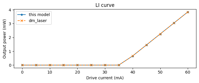
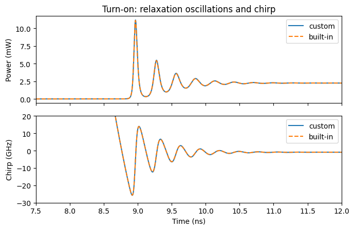
With nothing connected to the optical port the injection term is inactive and the model is a standard directly modulated laser. Two quick checks establish its operating point: the light-current characteristic locates the threshold near 36 mA, and a current step from below to above threshold shows the turn-on delay and the relaxation oscillations that set the internal time scale of everything that follows. The response of the built-in dm_laser, which solves the same rate equations, is plotted for comparison.

time_step = 0.5e-12  # fine enough to resolve the relaxation oscillations


def bias_link(laser_comp, source_comp, name):
    # laser driven by a signal source, optical output exposed as "out"
    link = pf.Component(name)
    laser_ref = link.add_reference(laser_comp)
    source_ref = link.add_reference(source_comp)
    source_ref.connect("E0", laser_ref["E0"])
    link.add_port(laser_ref["P0"], "out")
    link.add_model(pf.CircuitModel(), "Circuit")
    return link


# LI curve: sweep the DC current and record the settled output power
builtin_laser = pfa.dm_laser(seed=0)  # built-in laser, plotted for comparison
source_c = pfa.signal_source(amplitude=0, offset=0, seed=1)  # DC current source
source_b = pfa.signal_source(amplitude=0, offset=0, seed=1)
link_c = bias_link(laser, source_c, "li_custom")
link_b = bias_link(builtin_laser, source_b, "li_builtin")

currents = np.linspace(0, 60e-3, 13)  # 0 to 60 mA
li = {"custom": [], "built-in": []}
for current in currents:
    for tag, src, link in [("custom", source_c, link_c), ("built-in", source_b, link_b)]:
        src.update(offset=current * np.sqrt(z0))  # current I maps to amplitude I sqrt(z0)
        ts = link.setup_time_stepper(
            time_step=time_step, carrier_frequency=f0, show_progress=False
        )
        # run 5 ns and read the complex envelope at the output port
        a = ts.step(steps=10000, time_step=time_step, show_progress=False)["out@0"]
        li[tag].append(np.abs(a[-2000:]).mean() ** 2)  # settled power (last 1 ns)

fig, ax = plt.subplots(figsize=(7, 3), tight_layout=True)
ax.plot(currents * 1e3, np.array(li["custom"]) * 1e3, "o-", ms=4, label="this model")
ax.plot(currents * 1e3, np.array(li["built-in"]) * 1e3, "x--", ms=6, label="dm_laser")
ax.set(xlabel="Drive current (mA)", ylabel="Output power (mW)", title="LI curve")
_ = ax.legend()

# current step from 20 mA (below threshold) to 50 mA after an 8 ns settling time
i_low, i_high = 20e-3, 50e-3
num_steps = 30000
t = np.arange(num_steps) * time_step
traces = {}
for tag, laser_comp in [("custom", laser), ("built-in", builtin_laser)]:
    # slow trapezoid: hold 20 mA for 8 ns, then a sharp step to 50 mA
    src = pfa.signal_source(
        frequency=0.05e9,  # 20 ns period, only the first edge matters here
        offset=i_low * np.sqrt(z0),
        amplitude=(i_high - i_low) * np.sqrt(z0),
        waveform="trapezoid",
        width=0.9,
        rise=0.001,
        fall=0.001,
        start=8e-9,  # settle at the low bias first, then step
        seed=1,
    )
    link = bias_link(laser_comp, src, f"step_{tag}")
    ts = link.setup_time_stepper(
        time_step=time_step, carrier_frequency=f0, show_progress=False
    )
    traces[tag] = ts.step(steps=num_steps, time_step=time_step, show_progress=False)["out@0"]

fig, (ax1, ax2) = plt.subplots(2, 1, figsize=(7, 4.6), sharex=True, tight_layout=True)
for tag, ls in [("custom", "-"), ("built-in", "--")]:
    a = traces[tag]
    ax1.plot(t * 1e9, np.abs(a) ** 2 * 1e3, ls, label=tag)
    # chirp = d(envelope phase)/dt, the instantaneous frequency deviation
    chirp = np.gradient(np.unwrap(np.angle(a)), time_step) / (2 * np.pi)
    ax2.plot(t * 1e9, chirp / 1e9, ls, label=tag)
ax1.set(ylabel="Power (mW)", title="Turn-on: relaxation oscillations and chirp",
        xlim=(7.5, 12))
# below threshold the gain sits far under the cavity loss, which the phase equation
# turns into a large frequency offset; the limits frame the chirp after turn-on
ax2.set(xlabel="Time (ns)", ylabel="Chirp (GHz)", xlim=(7.5, 12), ylim=(-30, 20))
ax1.legend()
_ = ax2.legend()

The External Cavity as a Circuit

The feedback path is built from two stock elements:

• A mirror: a TerminationModel with a complex reflection coefficient sets both the feedback strength \(r_\text{ext} = \lvert r \rvert\) and, through its phase, the feedback phase.

• A waveguide: straight provides the propagation delay \(\tau = 2 L n_g / c_0\) and the round-trip envelope phase \(2 \cdot 2\pi f_0 n_\text{eff} L / c_0\).

Warning. The default time stepper of the waveguide model fits the S matrix with a pole-residue expansion, and the automatic delay extraction reads the phase slope on the sampled frequency grid. The default grid spans the carrier plus or minus 1 THz with 20 GHz spacing, so delays beyond \(1/(2\,\Delta f) = 25\) ps alias and are silently dropped. For delay lines, either pass a frequencies grid finer than \(1/(2\tau)\) or attach an AnalyticWaveguideTimeStepper, which implements the group delay exactly as an integer number of time steps. Feedback dynamics generate broad spectra, so this example uses the analytic stepper.

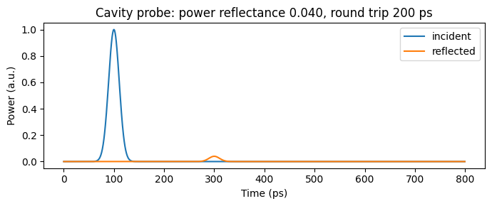
A short pulse reflected off the assembled cavity shows the two quantities that matter for the feedback problem: the round-trip amplitude and the round-trip delay.

# external cavity for the long-cavity study: 200 ps round trip
tau_ext = 200e-12
n_eff_wg, n_g_wg = 2.4, 4.0
wg_length = tau_ext * c_0 / (2 * n_g_wg) * 1e6  # one-way length in um
r_ext_probe = 0.2  # mirror used for the probe


def cavity_waveguide(length):
    wg = pfa.straight(length=length, n_eff=n_eff_wg, n_group=n_g_wg, reference_frequency=f0)
    # exact delay-line stepper instead of the fitted default (see warning above)
    wg.active_model.time_stepper = pf.AnalyticWaveguideTimeStepper(
        n_eff=n_eff_wg, length=length, n_group=n_g_wg
    )
    return wg


def mirror(r):
    # one-port mirror: complex r sets the feedback strength and phase
    return pf.TerminationModel(r=r).black_box_component(
        pf.virtual_port_spec(), name="Mirror"
    )


# one-port cavity: waveguide with the mirror at the far end
cavity = pf.Component("external_cavity")
wg_ref = cavity.add_reference(cavity_waveguide(wg_length))
mr_ref = cavity.add_reference(mirror(r_ext_probe))
mr_ref.connect("P0", wg_ref["P1"])
cavity.add_port(wg_ref["P0"], "in")  # probe port at the near end
cavity.add_model(pf.CircuitModel(), "Circuit")

# reflect a short gaussian envelope pulse off the cavity
num_probe = 1600
t_probe = np.arange(num_probe) * time_step
pulse = np.exp(-0.5 * ((t_probe - 100e-12) / 15e-12) ** 2).astype(complex)
ts = cavity.setup_time_stepper(time_step=time_step, carrier_frequency=f0, show_progress=False)
# inject the pulse into the exposed port; the output on the same port is the reflection
refl = ts.step(
    inputs=pf.TimeSeries(time_step=time_step, values={"in@0": pulse}),
    show_progress=False,
).values["in@0"]

fig, ax = plt.subplots(figsize=(7, 3), tight_layout=True)
ax.plot(t_probe * 1e12, np.abs(pulse) ** 2, label="incident")
ax.plot(t_probe * 1e12, np.abs(refl) ** 2, label="reflected")
ax.set(xlabel="Time (ps)", ylabel="Power (a.u.)",
       title=f"Cavity probe: power reflectance {np.abs(refl).max()**2:.3f}, "
             f"round trip {tau_ext*1e12:.0f} ps")
_ = ax.legend()

Closing the Loop: from Stable Emission to Coherence Collapse

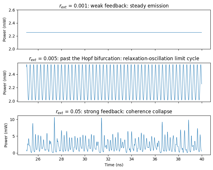
Connecting the cavity to the laser closes the feedback loop. The circuit has no exposed optical port: the laser output is observed with a monitor on its port. The feedback strength is the Lang-Kobayashi rate \(\kappa = \kappa_c\, r_\text{ext}\), swept here through the mirror reflectivity at a fixed cavity length. For this laser (\(r_2 = 0.556\), \(\tau_\text{in} = 7.1\) ps, a typical 300 um Fabry-Perot diode) \(\kappa_c = 1.8 \times 10^{11}\) 1/s.

The sequence of behaviors follows the feedback regimes of Tkach and Chraplyvy [2]:

• At weak feedback the laser remains steady; the emission frequency shifts as the laser locks to an external-cavity mode.

• When the feedback rate overcomes the relaxation-oscillation damping, the relaxation oscillations undamp (a Hopf bifurcation) and the output develops a gigahertz intensity oscillation.

• At strong feedback the dynamics become chaotic: coherence collapse, with intensity fluctuations of order the mean power and an optical spectrum broadened by tens of gigahertz. This is regime IV, the state that back-reflection specifications and optical isolators exist to avoid.

# coupling rate kappa_c for r2 = 0.556 and tau_in = 7.06 ps (300 um diode)
kc = (1 - 0.556**2) / (0.556 * 7.06e-12)


def feedback_loop(r_ext):
    # closed loop: laser -> waveguide -> mirror (no exposed optical port)
    loop = pf.Component(f"loop_{r_ext:.0e}")
    # laser with injection enabled, biased at 50 mA by a DC source
    laser_ref = loop.add_reference(feedback_laser(feedback_coupling_rate=kc))
    source_ref = loop.add_reference(
        pfa.signal_source(amplitude=0, offset=50e-3 * np.sqrt(z0), seed=1)
    )
    source_ref.connect("E0", laser_ref["E0"])
    # external cavity: waveguide from the laser port to the mirror
    wg_ref = loop.add_reference(cavity_waveguide(wg_length))
    wg_ref.connect("P0", laser_ref["P0"])
    mr_ref = loop.add_reference(mirror(r_ext))
    mr_ref.connect("P0", wg_ref["P1"])
    loop.add_model(pf.CircuitModel(), "Circuit")
    return loop, laser_ref


# display one assembled loop
loop_demo, _ = feedback_loop(5e-3)
viewer(loop_demo)

# sweep the mirror reflectivity across the Hopf bifurcation into chaos
r_values = [1e-4, 1e-3, 3e-3, 5e-3, 2e-2, 5e-2]
num_steps = 80000  # 40 ns at 0.5 ps per step
t = np.arange(num_steps) * time_step
tail = slice(num_steps - 30000, None)  # settled part used for statistics
loops = {}
for r_ext in r_values:
    loop, laser_ref = feedback_loop(r_ext)
    # a monitor on the laser port records the emitted and the returning wave
    ts = loop.setup_time_stepper(
        time_step=time_step, carrier_frequency=f0, show_progress=False,
        time_stepper_kwargs={"monitors": {"laser": laser_ref["P0"]}},
    )
    out = ts.step(steps=num_steps, time_step=time_step, show_progress=False)
    # keep the emitted wave: the direction with the larger mean power
    a_plus, a_minus = out.values["laser@0+"], out.values["laser@0-"]
    emitted = a_plus if np.mean(np.abs(a_plus) ** 2) > np.mean(np.abs(a_minus) ** 2) else a_minus
    loops[r_ext] = emitted

# time traces for three representative feedback levels
fig, axes = plt.subplots(3, 1, figsize=(7.5, 6), sharex=True, tight_layout=True)
for ax, r_ext, label in [
    (axes[0], 1e-3, "weak feedback: steady emission"),
    (axes[1], 5e-3, "past the Hopf bifurcation: relaxation-oscillation limit cycle"),
    (axes[2], 5e-2, "strong feedback: coherence collapse"),
]:
    p = np.abs(loops[r_ext]) ** 2 * 1e3
    ax.plot(t[tail] * 1e9, p[tail], lw=0.8)
    ax.set(ylabel="Power (mW)", title=f"$r_{{ext}}$ = {r_ext:g}: {label}")
axes[0].set_ylim(2.0, 2.6)  # steady emission: avoid an offset-notation axis
axes[0].ticklabel_format(useOffset=False, axis="y")
axes[2].set(xlabel="Time (ns)")
plt.show()

# oscillation amplitude vs feedback strength: the Hopf threshold stands out
fig, (ax1, ax2) = plt.subplots(1, 2, figsize=(9.5, 3.4), tight_layout=True)
stds = [(np.abs(loops[r]) ** 2)[tail].std() * 1e3 for r in r_values]
ax1.loglog(r_values, np.maximum(stds, 1e-9), "o-")
ax1.set(xlabel="Mirror reflectivity $r_{ext}$", ylabel="Power std (mW)",
        title="Onset of intensity oscillations")

# optical spectra of the same three states shown in the time traces:
# discrete external-cavity lines appear, then dissolve into a broad pedestal
freqs = np.fft.fftshift(np.fft.fftfreq(len(t[tail]), time_step))
for r_ext in [1e-3, 5e-3, 5e-2]:
    # spectrum of the complex envelope = optical spectrum around the carrier
    spec = np.fft.fftshift(np.abs(np.fft.fft(loops[r_ext][tail])) ** 2)
    ax2.semilogy(freqs / 1e9, spec / spec.max(), lw=0.8, label=f"$r_{{ext}}$ = {r_ext:g}")
ax2.set(xlabel="Frequency offset (GHz)", ylabel="Optical spectrum (norm.)",
        xlim=(-30, 30), ylim=(1e-9, 2), title="Coherence collapse")
_ = ax2.legend(fontsize=8)

Short-Cavity Regime: Regular Pulse Packages

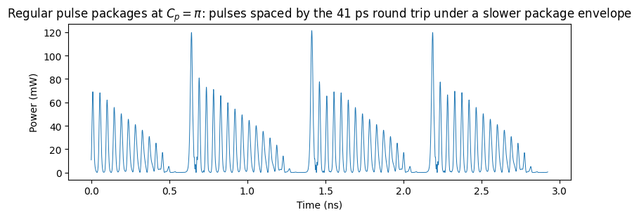
When the external round trip is shorter than the relaxation-oscillation period the dynamics change character. Heil et al. studied this regime experimentally and with the Lang-Kobayashi equations [3, 4] and found a robust state built around regular pulse packages (RPP): bursts of pulses spaced by the cavity round trip, repeating with a slower envelope period, highly sensitive to the feedback phase \(C_p\).

Their model uses dimensionless parameters. The table below maps the values of Ref. [4] (Figs. 5 to 7) onto this circuit; time is measured in photon lifetimes, so \(T = \tau_n / \tau_p\) fixes \(\tau_p\), the pump parameter \(P\) fixes the drive current, and the feedback strength \(\eta = \kappa \tau_p\) fixes the product of coupling rate and mirror reflectivity.

Ref. [4]	Value	Physical quantity here
\(T\)	1710	\(\tau_p = \tau_n / T = 0.58\) ps
\(P\)	0.8	\(I = 152\) mA \(= 2.04\, I_\text{th}\)
\(\tau\)	70	round trip \(= 41\) ps (1.5 mm of on-chip path)
\(\eta\)	0.115	\(\kappa_c\, r_\text{ext} = 2.0 \times 10^{11}\) 1/s
\(\alpha\)	5.0	linewidth enhancement factor
\(C_p\)	swept	round-trip envelope phase, set by the tuner voltage

Two details of the mapping: the reference model has no gain compression and no spontaneous emission, so those are set to (numerically) zero; and the feedback facet is antireflection coated in the experiment, consistent with the larger coupling rate used here (\(r_2 = 0.32\)).

The feedback phase is actuated by a phase tuner inside the cavity: a 1 mm phase_modulator with \(V_\pi L = 0.8\) V cm. Light passes it twice per round trip, so the phase shifts by \(2\pi V / V_\pi\) per round trip and one \(V_\pi / 2\) of drive covers a full cycle of \(C_p\), with the delay unchanged. All lengths are chosen so that every delay is an exact multiple of the time step.

# dimensionless targets from Ref. [4]
alpha_h = 5.0
t_ratio = 1710.0
p_pump = 0.8
tau_dim = 70.0
eta_fb = 0.115

# laser parameters mapped to physical values
tau_n = 1.0e-9  # carrier lifetime, sets the time unit of Ref. [4] (1/gamma)
tau_p = tau_n / t_ratio  # photon lifetime from T = tau_n / tau_p: 0.585 ps
n_tr = 1.1e24  # transparency carrier density (default laser value)
vg_a0 = c_0 / 3.53 * 2.5e-20  # v_g * a0 of the laser model
gam = 0.4  # confinement factor
v_a = 1.5e-16  # active volume (m^3)
# threshold carrier density: where modal gain equals the cavity loss 1/tau_p
n_th = n_tr + 1.0 / (gam * vg_a0 * tau_p)
# drive current: threshold current plus the excess pump set by P
i_heil = q_e * v_a * (n_th / tau_n + 2 * p_pump / (tau_n * tau_p * gam * vg_a0))

# feedback coupling: eta = tau_p * kappa_c * r_ext fixes the product of the
# facet coupling rate (AR-coated facet, r2 = 0.32) and the mirror reflectivity
r2_ar = 0.32
kc_heil = (1 - r2_ar**2) / (r2_ar * 7.06e-12)  # kappa_c for the AR facet
r_ext_heil = eta_fb / tau_p / kc_heil  # mirror reflectivity: 0.49

# time step: 10 steps per photon lifetime; round trip = 70 tau_p = 700 steps
dt = 0.1 * tau_p

# phase tuner: 1 mm, V_pi L = 0.8 V cm; its length is chosen so that the
# group delay is exactly 240 time steps (delays must be integer steps)
v_pil = 8000.0  # V_pi L in V um (0.8 V cm)
n_g_pm = 4.2  # tuner group index
pm_steps = 240
pm_length = pm_steps * dt * c_0 / n_g_pm * 1e6  # um
v_pi = v_pil / pm_length  # 8 V for this length

# waveguide making up the rest of the 350-step one-way path
wg_steps = int(round(tau_dim * tau_p / dt / 2)) - pm_steps  # 350 - 240 = 110 steps
wg_heil_length = wg_steps * dt * c_0 / n_g_wg * 1e6  # um

print(f"tau_p = {tau_p*1e12:.3f} ps, I = {i_heil*1e3:.1f} mA, "
      f"r_ext = {r_ext_heil:.2f}, V_pi = {v_pi:.1f} V")
print(f"tuner {pm_length:.0f} um + waveguide {wg_heil_length:.0f} um: "
      f"round trip {2*(pm_steps+wg_steps)*dt*1e12:.2f} ps")


def phase_tuner():
    return pfa.phase_modulator(
        length=pm_length, n_eff=2.4, n_group=n_g_pm, reference_frequency=f0,
        v_piL=v_pil, z0=z0, f_3dB=0,
    )


# calibrate the static round-trip phase with a pulse probe, then cancel it with the
# mirror phase so that C_p = (2 pi / v_pi) * V exactly
probe = pf.Component("heil_cavity_probe")
# same cavity as the loop below, with the laser replaced by a probe port
pm_ref = probe.add_reference(phase_tuner())
wg_ref = probe.add_reference(cavity_waveguide(wg_heil_length))
mr_ref = probe.add_reference(mirror(r_ext_heil))
src_ref = probe.add_reference(pfa.signal_source(amplitude=0, offset=0, seed=1))
src_ref.connect("E0", pm_ref["E0"])  # tuner held at 0 V
wg_ref.connect("P0", pm_ref["P1"])
mr_ref.connect("P0", wg_ref["P1"])
probe.add_port(pm_ref["P0"], "in")
probe.add_model(pf.CircuitModel(), "Circuit")

# reflect a short pulse and read the round-trip phase from the complex ratio
num_probe = 2 * (pm_steps + wg_steps) + 3000
t_pp = np.arange(num_probe) * dt
pulse = np.exp(-0.5 * ((t_pp - 40e-12) / 8e-12) ** 2).astype(complex)
ts = probe.setup_time_stepper(time_step=dt, carrier_frequency=f0, show_progress=False)
refl = ts.step(
    inputs=pf.TimeSeries(time_step=dt, values={"in@0": pulse}), show_progress=False
).values["in@0"]
mirror_phase = -np.angle(refl.sum() / pulse.sum())  # cancels the static phase
print(f"mirror phase offset: {mirror_phase:+.4f} rad")

tau_p = 0.585 ps, I = 152.2 mA, r_ext = 0.49, V_pi = 8.0 V
tuner 1002 um + waveguide 482 um: round trip 40.94 ps
mirror phase offset: -2.5882 rad

With the cavity calibrated, the loop is assembled once and stepped in segments: the tuner voltage is fed as a staircase, so the attractor state carries over from one feedback phase to the next, the same continuation protocol as in Ref. [4]. First a single run at \(C_p = \pi\) shows the regular pulse packages themselves.

def heil_loop():
    # closed loop: laser -> phase tuner -> waveguide -> mirror
    loop = pf.Component("heil_loop")
    # laser mapped to the reference parameter set (see the table above)
    laser_ref = loop.add_reference(
        feedback_laser(
            spontaneous_emission_factor=1e-8,  # tiny seed, the reference model has none
            gain_compression_factor=0.0,  # the reference model has none
            photon_lifetime=tau_p,
            linewidth_enhancement_factor=alpha_h,
            feedback_coupling_rate=kc_heil,
        )
    )
    # DC bias at the mapped pump current
    source_ref = loop.add_reference(
        pfa.signal_source(amplitude=0, offset=i_heil * np.sqrt(z0), seed=1)
    )
    source_ref.connect("E0", laser_ref["E0"])
    # cavity elements, in order from the laser to the mirror
    pm_ref = loop.add_reference(phase_tuner())
    wg_ref = loop.add_reference(cavity_waveguide(wg_heil_length))
    mr_ref = loop.add_reference(mirror(r_ext_heil * np.exp(1j * mirror_phase)))
    pm_ref.connect("P0", laser_ref["P0"])
    wg_ref.connect("P0", pm_ref["P1"])
    mr_ref.connect("P0", wg_ref["P1"])
    # the tuner drive is the only exposed port: it will receive the C_p staircase
    loop.add_port(pm_ref["E0"], "vp")
    loop.add_model(pf.CircuitModel(), "Circuit")
    return loop, laser_ref


# display the assembled loop
heil_demo, _ = heil_loop()
viewer(heil_demo)

def heil_stepper():
    # time stepper with a monitor on the laser port (emitted + returning wave)
    loop, laser_ref = heil_loop()
    return loop.setup_time_stepper(
        time_step=dt, carrier_frequency=f0, show_progress=False,
        time_stepper_kwargs={"monitors": {"laser": laser_ref["P0"]}},
    )


def run_segment(ts, volt, num):
    # hold the tuner at a constant voltage for num steps; the internal state
    # persists between calls, so consecutive segments continue the same run
    out = ts.step(
        inputs=pf.TimeSeries(
            time_step=dt, values={"vp@0": np.full(num, volt / np.sqrt(z0), complex)}
        ),
        show_progress=False,
    )
    # return the emitted wave (the monitor direction with larger mean power)
    a_plus, a_minus = out.values["laser@0+"], out.values["laser@0-"]
    return a_plus if np.mean(np.abs(a_plus) ** 2) > np.mean(np.abs(a_minus) ** 2) else a_minus


# regular pulse packages at C_p = pi
ts = heil_stepper()
v_cp_pi = np.pi * v_pi / (2 * np.pi)  # tuner voltage for C_p = pi
run_segment(ts, v_cp_pi, 200000)  # discard the turn-on transient (20000 tau_p)
emitted = run_segment(ts, v_cp_pi, 50000)  # keep 5000 tau_p for the plot

t_rpp = np.arange(len(emitted)) * dt
fig, ax = plt.subplots(figsize=(8, 3.2), tight_layout=True)
ax.plot(t_rpp * 1e9, np.abs(emitted) ** 2 * 1e3, lw=0.7)
ax.set(xlabel="Time (ns)", ylabel="Power (mW)",
       title=r"Regular pulse packages at $C_p = \pi$: pulses spaced by the 41 ps "
             "round trip under a slower package envelope")
plt.show()

Bifurcation Scenario versus Feedback Phase

Finally, the tuner voltage is stepped so that \(C_p\) walks from \(+\pi\) down to \(-\pi\) and then back up. At each phase the first 5000 photon lifetimes are discarded and the extrema of the normalized field amplitude \(R/\sqrt{P} - 1\) are collected over the next 200; sweeping in both directions catches the hysteresis between coexisting states. This is the recipe behind Fig. 7 of Ref. [4], and the resulting diagram reproduces the cyclic scenario reported there:

• a steady plateau (the maximum-gain mode) for \(C_p \gtrsim 1.4\),

• a Hopf bifurcation near \(C_p \approx 1.3\) with a limit cycle that grows as the phase decreases,

• quasi-periodic (torus) bands below \(C_p \approx -1\),

• and the abrupt appearance of pulse packages near \(C_p \approx -1.9\), whose extrema fill a broad band; on the return sweep the pulse packages persist well into the region where the steady mode also exists before the laser falls back onto it.

# conversion from monitor amplitude (sqrt W) to the normalized field amplitude
c_p_cal = 0.4 * h_planck * f0 * v_a / (2 * gam * tau_p)  # W per photon density
a2p = tau_n * vg_a0 / 2.0  # |A|^2 = a2p * p

cp_down = np.linspace(np.pi, -np.pi, 97)
n_transient = 50000  # 5000 photon lifetimes
n_record = 2000  # 200 photon lifetimes

diagram = []
for cp_values in [cp_down, cp_down[::-1]]:  # sweep down, then back up
    ts = heil_stepper()  # fresh loop for each sweep direction
    # let the cold-started laser turn on and settle at the first phase value
    run_segment(ts, cp_values[0] * v_pi / (2 * np.pi), 150000)
    for cp in cp_values:
        volt = cp * v_pi / (2 * np.pi)  # staircase level for this C_p
        run_segment(ts, volt, n_transient)  # transient, discarded
        emitted = run_segment(ts, volt, n_record)  # recorded segment
        # monitor amplitude -> photon density -> normalized field amplitude
        r_norm = np.sqrt(a2p * np.abs(emitted) ** 2 / c_p_cal) / np.sqrt(p_pump) - 1.0
        # local maxima and minima of the recorded trace
        dm = np.diff(r_norm)
        idx_max = np.where((dm[:-1] > 0) & (dm[1:] <= 0))[0] + 1
        idx_min = np.where((dm[:-1] < 0) & (dm[1:] >= 0))[0] + 1
        extrema = np.concatenate([r_norm[idx_max], r_norm[idx_min]])
        if len(extrema) == 0:
            extrema = r_norm[-1:]  # steady state: keep the level itself
        diagram.append((cp, extrema))

fig, ax = plt.subplots(figsize=(8, 5), tight_layout=True)
for cp, extrema in diagram:
    if len(extrema) > 60:
        extrema = extrema[:: len(extrema) // 60]
    ax.plot(np.full(len(extrema), cp), extrema, ".", color="k", ms=1.4, alpha=0.6)
ax.set(xlabel="Feedback phase $C_p$", ylabel=r"Field amplitude $R/\sqrt{P} - 1$",
       xlim=(-np.pi, np.pi), ylim=(-1.05, 2.5),
       title="Extrema of the field amplitude vs feedback phase, compare with "
             "Fig. 7 of Ref. [4]")
plt.show()

Conclusion

The laser built here is not a special case: it is an ordinary PhotonForge model. Every model in a circuit provides its dynamics through the same TimeStepper interface, so a user-defined subclass that implements setup_state, keys, and step_single enters a simulation on the same footing as the built-in lasers, modulators, and photodiodes: it can be parameterized, driven by sources, observed with monitors, and wired into any topology, while the circuit stepper takes care of every connection around it. Writing one is a matter of typing in the device physics, as done here and in the self-pulsing microring example.

That flexibility is what carried this study:

• The Lang-Kobayashi delayed term was never written in this notebook. The laser model only knows how incident light couples into its rate equations; the delay, strength, and phase of the feedback all come from ordinary circuit elements. Any modification of the feedback path (two mirrors, a filtered reflector, another laser instead of the mirror) is a change of netlist, not of model code.

• The same setup quantifies engineering questions directly: the Hopf threshold found in the reflectivity sweep is the tolerable back-reflection level for this laser, and its dependence on bias, linewidth enhancement factor, and cavity length can be swept with a few lines.

• The two knobs of the short-cavity experiment, feedback strength and feedback phase, map onto a mirror parameter and a tuner voltage. Stepping the tuner voltage while the simulation runs preserves the attractor, which is what resolves hysteresis between coexisting states.

The same recipe extends beyond this example: any device whose physics can be written as differential equations driven by its port signals, from saturable absorbers to mutually coupled lasers, can be dropped into a PhotonForge circuit the same way and explored against everything else in the model library.