Time Delay

Propagation takes time: light crosses a fiber patch cord, an RF drive travels down a cable, and mismatched path lengths turn into skew between signals. Instead of modeling each of these with its own component, the DelayedTimeStepper wraps any existing time stepper and delays its inputs, its outputs, or both:

• input_delay and output_delay set default delays for all ports,

• per-port overrides are passed at setup time as input_delays / output_delays dictionaries keyed by port name, which makes skews between ports possible.

Delays are realized as whole numbers of time steps, so the time step should divide the delays of interest. This guide wraps an existing model to shift its response, applies a per-port override, and closes with the classic circuit built from a delay: the delay-line interferometer.

Setup

import matplotlib.pyplot as plt
import numpy as np
import photonforge as pf
import photonforge.abstract as pfa

viewer = pf.live_viewer.LiveViewer()

LiveViewer started at http://localhost:56831

tech = pf.basic_technology()
pf.config.default_technology = tech

f0 = pf.C_0 / 1.55
time_step = 1e-12

Delaying an Existing Model

Every model carries its time stepper in its time_stepper attribute, so adding a delay is a one-line wrap: replace the stepper with a DelayedTimeStepper around it. Here a Bessel low-pass filter gets 50 ps of output delay, standing in for the cable between a driver and its load, and its impulse response simply shifts by that amount relative to an unmodified copy.

num_steps = 512
t = np.arange(num_steps) * time_step
impulse = np.zeros(num_steps)
impulse[0] = 1.0

# An unmodified filter for reference
filter_reference = pfa.filter(family="bessel", f_cutoff=20e9, order=4)

# An identical filter whose stepper is wrapped with 50 ps of output delay
filter_delayed = pfa.filter(family="bessel", f_cutoff=20e9, order=4, insertion_loss=1e-9)
model = filter_delayed.active_model
model.time_stepper = pf.DelayedTimeStepper(model.time_stepper, output_delay=50e-12)

fig, ax = plt.subplots(figsize=(7, 3), tight_layout=True)
for label, component in [("Original", filter_reference), ("50 ps output delay", filter_delayed)]:
    # Run directly on the component and inject the impulse on its input port
    time_stepper = component.setup_time_stepper(
        time_step=time_step, carrier_frequency=f0, show_progress=False
    )
    out = time_stepper.step(inputs=pf.TimeSeries({"E0@0": impulse}, time_step), show_progress=False)
    ax.plot(t * 1e12, np.real(out["E1@0"]), label=label)
ax.set(xlabel="Time (ps)", ylabel="Output", xlim=(0, 200))
_ = ax.legend(fontsize=8)

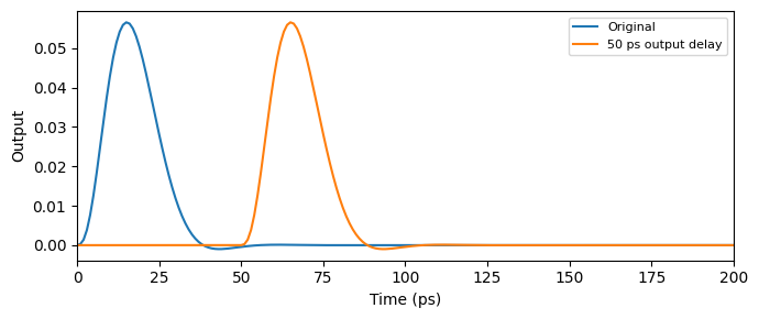
A detail worth knowing: two abstract components created with identical arguments are the same shared object, so the delayed copy above is created with a vanishingly small insertion_loss to make it a distinct component before its stepper is replaced.

Per-Port Delays

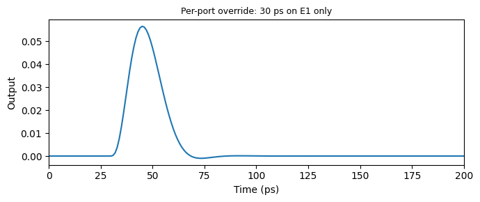
The constructor delays apply to all ports; individual ports are overridden at setup time through time_stepper_kwargs. Here the same wrapper carries no default delay, and only the output port E1 receives 30 ps, the pattern used for modeling skew, for example between the two drives of a differential circuit.

filter_skew = pfa.filter(family="bessel", f_cutoff=20e9, order=4, insertion_loss=2e-9)
model = filter_skew.active_model
model.time_stepper = pf.DelayedTimeStepper(model.time_stepper)

# Per-port override: only E1 is delayed, passed at setup time
time_stepper = filter_skew.setup_time_stepper(
    time_step=time_step,
    carrier_frequency=f0,
    show_progress=False,
    time_stepper_kwargs={"output_delays": {"E1@0": 30e-12}},
)
out = time_stepper.step(inputs=pf.TimeSeries({"E0@0": impulse}, time_step), show_progress=False)

fig, ax = plt.subplots(figsize=(7, 3), tight_layout=True)
ax.plot(t * 1e12, np.real(out["E1@0"]))
ax.set(xlabel="Time (ps)", ylabel="Output", xlim=(0, 200))
_ = ax.set_title("Per-port override: 30 ps on E1 only", fontsize=9)

Application: a Delay-Line Interferometer

A splitter, two paths with a differential delay \(\tau\), and a combiner form a delay-line interferometer, the building block behind DPSK demodulators and periodic comb filters. We build it from two 3 dB directional_coupler components with identity blocks as the arms (unity-gain, noiseless optical_amplifier components), wrapping one arm’s stepper with \(\tau = 10\) ps.

Because abstract components are schematic symbols, the delayed arm cannot always be closed geometrically; add_virtual_connection forces its netlist connection to the combiner regardless of the symbol positions. In this particular circuit the two arm symbols happen to have identical footprints, so the delayed arm’s output port lands exactly on the combiner port and touching ports are connected automatically; the explicit virtual connection keeps the netlist correct for arms of any size.

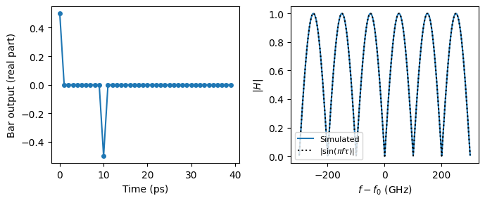
A single injected impulse tells the whole story: the bar port receives the through-path copy at \(t = 0\) and the delayed copy with opposite sign at \(t = \tau\), and the Fourier transform of that impulse pair is the comb response \(\lvert H(f) \rvert = \lvert \sin(\pi f \tau) \rvert\) with a free spectral range of \(1 / \tau = 100\) GHz.

tau = 10e-12

# Identity arms: unity-gain noiseless amplifiers (distinct seeds keep them separate)
arm_through = pfa.optical_amplifier(gain=0, seed=1)
arm_delayed = pfa.optical_amplifier(gain=0, seed=2)
model = arm_delayed.active_model
model.time_stepper = pf.DelayedTimeStepper(model.time_stepper, output_delay=tau)

# Splitter, both arms, combiner, chained in signal-flow order
interferometer = pf.Component("delay_line_interferometer")
splitter_ref = interferometer.add_reference(pfa.directional_coupler())
arm_through_ref = interferometer.add_reference(arm_through)
arm_delayed_ref = interferometer.add_reference(arm_delayed)
combiner_ref = interferometer.add_reference(pfa.directional_coupler())
termination_ref = interferometer.add_reference(pfa.optical_termination())
arm_through_ref.connect("P0", splitter_ref["P2"])
arm_delayed_ref.connect("P0", splitter_ref["P3"])
combiner_ref.connect("P0", arm_through_ref["P1"])
# The delayed arm's output is wired to the combiner explicitly, independent of geometry
interferometer.add_virtual_connection(arm_delayed_ref, "P1", combiner_ref, "P1")
termination_ref.connect("P0", splitter_ref["P1"])
interferometer.add_port(splitter_ref["P0"], "in")
interferometer.add_port(combiner_ref["P2"], "bar")
interferometer.add_port(combiner_ref["P3"], "cross")
interferometer.add_model(pf.CircuitModel(), "Circuit")
viewer(interferometer)

num_steps = 4096
t = np.arange(num_steps) * time_step
impulse_opt = np.zeros(num_steps, complex)
impulse_opt[0] = 1.0

time_stepper = interferometer.setup_time_stepper(
    time_step=time_step, carrier_frequency=f0, show_progress=False
)
out = time_stepper.step(inputs=pf.TimeSeries({"in@0": impulse_opt}, time_step), show_progress=False)
bar = out["bar@0"]

# Impulse pair and its spectrum, with the analytic comb for reference
h = np.abs(np.fft.fft(bar))
freq = np.fft.fftfreq(num_steps, time_step)
order = np.argsort(freq)

fig, (ax1, ax2) = plt.subplots(1, 2, figsize=(7, 3), tight_layout=True)
ax1.plot(t[:40] * 1e12, np.real(bar[:40]), "o-", markersize=4)
ax1.set(xlabel="Time (ps)", ylabel="Bar output (real part)")
band = np.abs(freq[order]) < 300e9
ax2.plot(freq[order][band] / 1e9, h[order][band], label="Simulated")
ax2.plot(freq[order][band] / 1e9, np.abs(np.sin(np.pi * freq[order][band] * tau)), "k:",
         label="$|\\sin(\\pi f \\tau)|$")
ax2.set(xlabel="$f - f_0$ (GHz)", ylabel="$|H|$")
_ = ax2.legend(fontsize=8)

Summary

• DelayedTimeStepper wraps any time stepper and delays its inputs and outputs; the wrap is a one-line replacement of a model’s time_stepper attribute.

• input_delay / output_delay set defaults, and per-port input_delays / output_delays dictionaries passed through time_stepper_kwargs at setup model skews between ports.

• Delays are realized in whole time steps, so choose the time step to divide the delays that matter.

• A differential delay between two interferometer arms produces the classic delay-line interferometer with its \(\lvert \sin(\pi f \tau) \rvert\) comb response and \(1 / \tau\) free spectral range.

• For delays tied to physical propagation, the waveguide-like models (straight with its group index, or the propagation_length of a TwoPortModel) include the delay from their geometry; this wrapper is the tool when the delay is an independent parameter.