Nonlinear Ring Resonator

A microring resonator stores light for many round trips, so the power circulating in the ring is much larger than the power in the bus waveguide. At milliwatt input powers this circulating power changes the ring itself. In a silicon ring three mechanisms act on the resonance:

• Heating. Absorbed light raises the ring temperature, and the thermo-optic effect increases the refractive index. The resonance moves to longer wavelengths (lower frequencies) with a thermal time constant of tens to hundreds of nanoseconds.

• Two-photon absorption (TPA) and free carriers. Two photons together can excite an electron-hole pair in silicon. TPA adds loss that grows with intensity, and the generated free carriers add free-carrier absorption (FCA) and lower the refractive index through free-carrier dispersion (FCD). FCD moves the resonance to higher frequencies. The carriers recombine within nanoseconds.

• The Kerr effect. The refractive index follows the intensity instantaneously, \(\Delta n = n_2 I\). In silicon this is small against the other two, but it is the main nonlinearity of silicon nitride rings, which have no TPA.

Because the resonance moves with the power stored in the ring, and the stored power depends on where the resonance sits relative to the laser, the ring responds to its own light. This feedback causes optical bistability [1, 2] and, when a fast effect and a slow effect push in opposite directions, self-pulsing [3, 4].

RingTimeStepper includes all of these effects as optional arguments, and nonlinear_ring wraps it in a component with a single bus (two ports) or two buses (four ports), plus an optional heater port. This guide shows how to use them for thermo-optic bistability, heater tuning and self-pulsing in a silicon add-drop ring. The linear ring and its electro-optic modulation are covered in the Ring Resonator guide.

What the time stepper computes

The time stepper represents the ring as a delay line sampled at the time step, closed on itself through one coupler per bus. At every step it computes the power circulating in the ring, \(P_\mathrm{c}\), averaged over the delay line and summed over both directions of propagation, and from it the intensity \(I = P_\mathrm{c}/A_\mathrm{eff}\) for a nonlinear effective area \(A_\mathrm{eff}\).

The carrier density \(N\) and the temperature rise \(\Delta T\) are two state variables. The carriers are generated by TPA, one electron-hole pair for every two absorbed photons, and recombined with a lifetime \(\tau_\mathrm{c}\):

\[\frac{\mathrm{d}N}{\mathrm{d}t} = \frac{\Gamma\,\beta_\mathrm{TPA}\,I^2}{2 h\nu} - \frac{N}{\tau_\mathrm{c}(N)},\]

where \(\beta_\mathrm{TPA}\) is the TPA coefficient, \(\Gamma\) the fraction of the mode inside the silicon core, and \(h\nu\) the photon energy. The temperature follows Newton’s law of cooling, with a thermal time constant \(\tau_\mathrm{th}\) and a heat capacity \(C_\mathrm{th}\):

\[\frac{\mathrm{d}\Delta T}{\mathrm{d}t} = \frac{P_\mathrm{heat}}{C_\mathrm{th}} - \frac{\Delta T}{\tau_\mathrm{th}}.\]

The heat source \(P_\mathrm{heat}\) has two parts. The first is the absorbed optical power, which collects every loss mechanism that turns light into heat, integrated over the ring length \(L\). The second is the power \(V^2/R\) of an optional heater with resistance \(R\) driven with voltage \(V\):

\[P_\mathrm{heat} = \left(f_\mathrm{abs}\,\alpha + \Gamma\,\beta_\mathrm{TPA}\,I + \sigma_\mathrm{FCA} N\right) P_\mathrm{c}\,L + \frac{V^2}{R}.\]

Here \(\alpha\) is the linear propagation loss, \(f_\mathrm{abs}\) the fraction of it that is absorption rather than scattering, and \(\sigma_\mathrm{FCA}\) the FCA cross-section. In steady state the temperature rise is \(\Delta T = R_\mathrm{th} P_\mathrm{heat}\), with the thermal impedance \(R_\mathrm{th} = \tau_\mathrm{th}/C_\mathrm{th}\).

The model has a single thermal node. The whole heater power is delivered to it, with the same \(R_\mathrm{th}\) and \(\tau_\mathrm{th}\) as the optical absorption. The section on tuning with the heater shows how to describe a heater that is less efficient than that.

With \(P_\mathrm{c}\) held for one time step, both equations are linear, so the time stepper advances each by its exact exponential solution. The state then changes the effective index and the loss of every slice of the ring:

\[\Delta n = n_2 I + \sigma_\mathrm{FCD} N + \frac{\mathrm{d}n}{\mathrm{d}T}\Delta T, \qquad \Delta\alpha = \Gamma\,\beta_\mathrm{TPA}\,I + \sigma_\mathrm{FCA} N,\]

where \(\sigma_\mathrm{FCD}\) is the FCD coefficient, negative in silicon.

The arguments map onto these quantities as follows:

• effective_area is \(A_\mathrm{eff}\) in m². It is required by the Kerr, TPA and free-carrier terms. Leaving it as None disables all three.

• kerr_index is \(n_2\) in m²/W, and tpa_coefficient is \(\beta_\mathrm{TPA}\) in m/W.

• fca_cross_section is \(\sigma_\mathrm{FCA}\) in m², and fcd_coefficient is \(\sigma_\mathrm{FCD}\) in m³.

• confinement is \(\Gamma\). It scales the TPA loss and the carriers it generates, while \(n_2\) and the free-carrier coefficients are taken as values for the mode.

• carrier_lifetime is \(\tau_\mathrm{c}\), a constant in s or an Interpolator over the carrier density in m⁻³. The free-carrier terms need it.

• thermal_time_constant and thermal_capacity are \(\tau_\mathrm{th}\) in s and \(C_\mathrm{th}\) in J/K. Setting both enables self-heating, which acts through the thermo-optic coefficient dn_dT.

• absorbed_fraction is \(f_\mathrm{abs}\).

• heater_resistance is \(R\) in Ω. Setting it adds an electrical port whose voltage heats the ring.

A nonlinear ring has no S matrix, since its response depends on the signal. The component is used in time-domain simulations only. For the frequency response of the same ring at low power, use RingModel with the same geometry.

References

1. Almeida, V. R., and Lipson, M. “Optical bistability on a silicon chip.” Optics Letters 2004 29 (20), 2387-2389, doi: 10.1364/OL.29.002387.

2. Carmon, T., Yang, L., and Vahala, K. J. “Dynamical thermal behavior and thermal self-stability of microcavities.” Optics Express 2004 12 (20), 4742-4750, doi: 10.1364/OPEX.12.004742.

3. Johnson, T. J., Borselli, M., and Painter, O. “Self-induced optical modulation of the transmission through a high-Q silicon microdisk resonator.” Optics Express 2006 14 (2), 817-831, doi: 10.1364/OPEX.14.000817.

4. Borghi, M., Bazzanella, D., Mancinelli, M., and Pavesi, L. “On the modeling of thermal and free carrier nonlinearities in silicon-on-insulator microring resonators.” Optics Express 2021 29 (3), 4363-4377, doi: 10.1364/OE.413572.

Setup

We use a silicon add-drop ring with a 7 µm radius near 1550 nm, with the parameters of the ring studied by Borghi et al. [4]. Papers usually describe a ring by its quality factors. The class method pf.RingModel.parameters_from_q converts an intrinsic quality factor \(Q_\mathrm{i}\) and a coupling quality factor \(Q_\mathrm{e}\) per bus into the propagation_loss, kappa1 and kappa2 arguments, through the round-trip time \(T = n_g L / c\):

\[\gamma_\mathrm{i} = \frac{\omega_0}{2Q_\mathrm{i}}, \qquad \gamma_\mathrm{e} = \frac{\omega_0}{2Q_\mathrm{e}}, \qquad \lvert\kappa\rvert^2 = 2\gamma_\mathrm{e} T, \qquad \alpha = \frac{2\gamma_\mathrm{i}}{v_g}.\]

Here \(\gamma_\mathrm{i}\) and \(\gamma_\mathrm{e}\) are the decay rates of the field amplitude through loss and through each bus, and \(v_g = c/n_g\) is the group velocity. The ring is strongly overcoupled, \(Q_\mathrm{e} \ll Q_\mathrm{i}\), so most of the light on resonance reaches the drop port.

import matplotlib.pyplot as plt
import numpy as np
import photonforge as pf
import photonforge.abstract as pfa

# Open the live viewer to display the ring component
viewer = pf.live_viewer.LiveViewer()

# Use the basic technology for the abstract components
pf.config.default_technology = pf.basic_technology()

# Set the reference frequency at which the indices are quoted (Hz)
f0 = 192.88e12
omega0 = 2 * np.pi * f0

# Set the ring geometry
radius = 7.0  # Ring radius (um)
length = 2 * np.pi * radius  # Round-trip length (um)
n_eff = 2.55  # Effective index at f0
n_group = 4.4  # Group index

# Set the quality factors of the ring
q_intrinsic = 1.1e5  # Intrinsic quality factor
q_coupling = 1.4e4  # Coupling quality factor of each bus

# Convert the quality factors to propagation loss and bus couplings
coupling = pf.RingModel.parameters_from_q(
    f0,
    q_intrinsic=q_intrinsic,
    q_coupling=(q_coupling, q_coupling),
    length=length,
    n_group=n_group,
)
print(coupling)

# Collect the linear ring arguments shared by every model below
ring_kwargs = dict(
    n_eff=n_eff,
    n_group=n_group,
    length=length,
    reference_frequency=f0,
    **coupling,
)

# Compute the amplitude decay rates through loss and through each bus (1/s)
gamma_i = omega0 / (2 * q_intrinsic)
gamma_e = omega0 / (2 * q_coupling)
gamma = gamma_i + 2 * gamma_e
print(f"Loaded quality factor: {omega0 / (2 * gamma):.0f}")
print(f"Linewidth: {2 * gamma / (2 * np.pi) / 1e9:.1f} GHz")

LiveViewer started at http://127.0.0.1:45569. Call its 'stop()' method to free the port.
{'propagation_loss': np.float64(0.0007022482496981677), 'kappa1': 0.2363874718876598, 'kappa2': 0.2363874718876598}
Loaded quality factor: 6581
Linewidth: 29.3 GHz

The loaded linewidth, about 29 GHz, is the frequency scale of everything that follows: a nonlinearity matters once it moves the resonance by a sizeable fraction of it.

Locating the resonance

A ring resonates when the round-trip phase is a multiple of \(2\pi\). Each coupler adds a phase to the light that passes it, so the resonances do not fall exactly on the comb \(f_m = m c/(n L)\) set by the waveguide alone. The simplest way to find a resonance is to compute the drop spectrum of the linear ring with pf.RingModel, which uses the same coupler convention as the time stepper. The next cell computes the drop transmission over one free spectral range (FSR) and takes the maximum.

# Build the linear ring model and a component to evaluate it on
linear_model = pf.RingModel(**ring_kwargs)
linear_ring = linear_model.black_box_component(
    port_spec=pf.virtual_port_spec(classification="optical")
)

# Compute the free spectral range (Hz)
fsr = pf.C_0 / (n_group * length)
print(f"FSR: {fsr / 1e9:.0f} GHz")

# Scan one FSR around f0 and compute the drop transmission from P0 to P2
freqs = np.linspace(f0 - fsr / 2, f0 + fsr / 2, 20001)
s_matrix = linear_model.s_matrix(linear_ring, freqs, show_progress=False)
drop = np.abs(s_matrix[("P0@0", "P2@0")]) ** 2

# Take the drop maximum as the cold resonance frequency
f_res = freqs[np.argmax(drop)]
print(f"Resonance: {pf.C_0 / f_res * 1e3:.3f} nm, drop transmission {drop.max():.3f}")

FSR: 1549 GHz
Resonance: 1550.038 nm, drop transmission 0.887

Now we create the nonlinear ring. With only the linear arguments it behaves exactly as the linear ring. The component has four optical ports: P0 is the input, P1 the through port, P2 the drop port and P3 the add port.

A single component needs no surrounding circuit: setup_time_stepper returns its time stepper, and the input field is passed to step as a TimeSeries keyed by the input port, "P0@0". Field amplitudes are in \(\sqrt{\text{W}}\). The time step must resolve the two couplers, which sit half a round trip apart, so we use half the round-trip time. The next cell drives the ring with a weak CW input at several detunings from the resonance and compares the settled drop power with the frequency-domain spectrum.

# Create the nonlinear ring with the linear arguments only
ring = pfa.nonlinear_ring(**ring_kwargs)
viewer(ring)

# Set the time step to half a round trip, so each coupler has its own slice
round_trip = n_group * length / pf.C_0
time_step = round_trip / 2
print(f"Round trip: {round_trip * 1e12:.3f} ps")

# Set a weak CW input and a run long enough for the ring to settle
p_in = 1e-6  # Input power (W)
num_steps = 20000  # About 13 ns, hundreds of photon lifetimes

# Choose the detunings of the laser from the resonance (Hz)
detunings = np.linspace(-60e9, 60e9, 9)

drop_time = []
for detuning in detunings:
    # Run the ring with the carrier at the laser frequency
    time_stepper = ring.setup_time_stepper(
        time_step=time_step, carrier_frequency=f_res + detuning, show_progress=False
    )
    a_in = np.full(num_steps, np.sqrt(p_in), dtype=complex)
    outputs = time_stepper.step(
        inputs=pf.TimeSeries({"P0@0": a_in}, time_step), show_progress=False
    )

    # Read the settled drop transmission from the last sample
    drop_time.append(np.abs(outputs["P2@0"][-1]) ** 2 / p_in)

# Plot the frequency-domain drop spectrum and the time-domain points
fig, ax = plt.subplots(figsize=(7, 3), tight_layout=True)
ax.plot((freqs - f_res) / 1e9, drop, label="RingModel")
ax.plot(detunings / 1e9, drop_time, "o", label="nonlinear_ring, 1 µW")
ax.set(
    xlabel="Detuning from resonance (GHz)", ylabel="Drop transmission", xlim=(-100, 100)
)
ax.legend()
plt.show()

Round trip: 0.646 ps

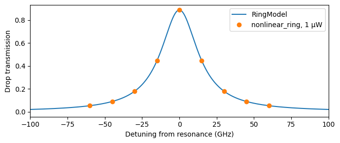
At 1 µW the nonlinear terms are negligible, and the time-domain points fall on the linear spectrum. The frequency-domain RingModel is therefore a convenient way to plan an experiment on the nonlinear ring: it gives the resonance and the linewidth directly.

Thermo-optic bistability

We first enable self-heating alone. Silicon has a thermo-optic coefficient \(\mathrm{d}n/\mathrm{d}T = 1.86\times10^{-4}\) K⁻¹. For the heat capacity of this small ring and a thermal time constant of 275 ns, Borghi et al. [4] give a thermal impedance \(R_\mathrm{th} = \tau_\mathrm{th}/C_\mathrm{th}\) of 36 K/mW. We leave effective_area unset, which turns off the Kerr, TPA and free-carrier terms, so heating is the only nonlinear effect.

Steady state. For a laser at frequency \(f_\mathrm{L}\), coupled-mode theory gives the energy \(U\) stored in the ring and the drop power:

\[U = \frac{2\gamma_\mathrm{e}\,P_\mathrm{in}}{\Delta^2 + \gamma^2}, \qquad P_\mathrm{drop} = 2\gamma_\mathrm{e}\,U, \qquad \gamma = \gamma_\mathrm{i} + 2\gamma_\mathrm{e},\]

where \(\Delta\) is the angular detuning of the laser from the heated resonance. The absorbed power is \(2\gamma_\mathrm{i} U\), so the temperature rise is \(\Delta T = 2\gamma_\mathrm{i} U R_\mathrm{th}\), and the heating moves the resonance by \(\delta f = -f_\mathrm{res}\,(\mathrm{d}n/\mathrm{d}T)\,\Delta T/n_g\). Together:

\[\Delta = 2\pi\left(f_\mathrm{L} - f_\mathrm{res} + \frac{f_\mathrm{res}}{n_g}\frac{\mathrm{d}n}{\mathrm{d}T}\Delta T\right).\]

These equations are implicit in \(U\), but they can be solved for the input power instead: choose \(\Delta T\), compute \(U\) and \(\Delta\), and then \(P_\mathrm{in} = U(\Delta^2 + \gamma^2)/ (2\gamma_\mathrm{e})\). For a laser on the red side of the resonance (\(f_\mathrm{L} < f_\mathrm{res}\)) this curve folds back on itself above a threshold power: over a range of input powers the ring has two stable states, a cold one with the resonance far from the laser and a hot one with the resonance pulled onto it. Which one the ring occupies depends on its history.

Time-domain sweep. The next cell runs the time stepper while it ramps the input power up and then down, with the laser 40 GHz below the cold resonance. It holds each power until the temperature has settled, reads the drop power, and plots it with the analytic steady state above for comparison. The steady states depend only on \(R_\mathrm{th}\), not on \(\tau_\mathrm{th}\). We therefore shorten \(\tau_\mathrm{th}\) to 2 ns and scale \(C_\mathrm{th}\) to keep \(R_\mathrm{th}\) at 36 K/mW, which makes each hold 140 times shorter and leaves the sweep unchanged. The real time constant returns in the next sections, where the dynamics matter.

# Set the thermal properties of the silicon ring
dn_dt = 1.86e-4  # Thermo-optic coefficient of silicon (1/K)
tau_th = 275e-9  # Thermal time constant (s)
c_th = 7.63e-12  # Heat capacity of the ring (J/K)
r_th = tau_th / c_th  # Thermal impedance (K/W)
print(f"Thermal impedance: {r_th / 1e3:.1f} K/mW")

# Shorten the thermal time constant and keep the thermal impedance for the sweep
tau_sweep = 2e-9  # Thermal time constant for the quasi-static sweep (s)
thermal_ring = pfa.nonlinear_ring(
    **ring_kwargs,
    dn_dT=dn_dt,
    thermal_time_constant=tau_sweep,
    thermal_capacity=tau_sweep / r_th,
)

# Place the laser 40 GHz below the cold resonance, on the red side
f_laser = f_res - 40e9

# Set up one time stepper for the whole sweep, so each power starts from the last state
time_stepper = thermal_ring.setup_time_stepper(
    time_step=time_step, carrier_frequency=f_laser, show_progress=False
)

# Hold each power for ten thermal time constants
hold_steps = int(10 * tau_sweep / time_step)

# Sweep the input power up and then back down (W)
p_sweep = np.linspace(0.05e-3, 2.5e-3, 50)
sweeps = {"Power up": p_sweep, "Power down": p_sweep[::-1]}

drop_sweep = {}
for name, powers in sweeps.items():
    values = []
    for power in powers:
        # Continue the same run at the next input power
        a_in = np.full(hold_steps, np.sqrt(power), dtype=complex)
        outputs = time_stepper.step(
            inputs=pf.TimeSeries({"P0@0": a_in}, time_step), show_progress=False
        )

        # Read the settled drop power
        values.append(np.abs(outputs["P2@0"][-1]) ** 2)
    drop_sweep[name] = np.array(values)

# Solve the steady state for the input power over a range of temperature rises (K)
delta_t = np.linspace(0, 120, 2000)
energy = delta_t / (2 * gamma_i * r_th)
detuning = 2 * np.pi * (f_laser - f_res + f_res / n_group * dn_dt * delta_t)
p_in_law = energy * (detuning**2 + gamma**2) / (2 * gamma_e)
p_drop_law = 2 * gamma_e * energy

# Plot both sweeps with the steady-state law
fig, ax = plt.subplots(figsize=(7, 3.2), tight_layout=True)
ax.plot(p_in_law * 1e3, p_drop_law * 1e3, "k:", label="Steady-state law")
ax.plot(p_sweep * 1e3, drop_sweep["Power up"] * 1e3, "o", ms=4, label="Power up")
ax.plot(
    p_sweep[::-1] * 1e3, drop_sweep["Power down"] * 1e3, "x", ms=5, label="Power down"
)
ax.set(
    xlabel="Input power (mW)", ylabel="Drop power (mW)", xlim=(0, 2.5), ylim=(0, 2.4)
)
ax.legend()
plt.show()

# Find the pair of powers between which each sweep jumps to the other branch
i_up = np.argmax(np.diff(drop_sweep["Power up"]))
i_down = np.argmin(np.diff(drop_sweep["Power down"]))
p_down = p_sweep[::-1]
print(
    f"Up sweep: jump between {p_sweep[i_up] * 1e3:.2f} and {p_sweep[i_up + 1] * 1e3:.2f} mW"
)
print(
    f"Down sweep: jump between {p_down[i_down] * 1e3:.2f} and {p_down[i_down + 1] * 1e3:.2f} mW"
)

Thermal impedance: 36.0 K/mW

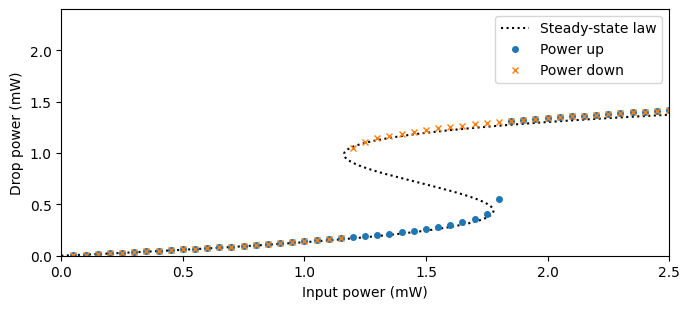
Up sweep: jump between 1.80 and 1.85 mW
Down sweep: jump between 1.20 and 1.15 mW

On the way up the ring stays on the cold branch: the laser sits on the tail of the resonance, little light is absorbed, and the resonance barely moves. At the end of that branch the heating pulls the resonance onto the laser, and the drop power jumps to the hot branch. On the way down the ring stays hot to much lower input powers, because the stored light keeps the resonance near the laser, until the hot branch ends and the ring falls back. Between the two jumps the ring is bistable, and the dotted law also shows the unstable middle branch that joins the two ends. The point just past the end of the cold branch is still on its way to the hot branch after ten time constants: close to the fold of the curve the ring settles slowly. The width of the loop grows with the detuning of the laser, and no loop forms for a laser close to or above the resonance.

Tuning with the heater

Rings are usually tuned with a resistive heater next to the waveguide. Setting heater_resistance adds an electrical port E0 to the component, and the voltage on it heats the ring with the power \(V^2/R\). The heater acts on the same temperature as the optical absorption, so it tunes the resonance with the efficiency

\[\frac{\delta f}{P_\mathrm{h}} = -\frac{f_\mathrm{res}}{n_g}\frac{\mathrm{d}n}{\mathrm{d}T} R_\mathrm{th}\]

and with the same time constant \(\tau_\mathrm{th}\).

In a real device this is an upper bound. Optical heat is released inside the silicon core, while a heater sits a micron or more away, and most of its power flows into the cladding and the substrate without passing through the waveguide. If only a fraction \(\eta\) of the heater power effectively reaches the ring, set heater_resistance to \(R/\eta\). The time stepper then applies \(\eta V^2/R\), and the tuning efficiency above is multiplied by \(\eta\). Obtain \(\eta\) as the ratio of the measured heater tuning efficiency to the value above, or from a thermal simulation of the cross-section.

The electrical input of the time stepper is a wave amplitude in \(\sqrt{\text{W}}\), related to the voltage by \(V = \mathrm{Re}(a)\sqrt{z_0}\), so a voltage \(V\) is injected as the amplitude \(V/\sqrt{z_0}\).

The next cell uses the real thermal time constant of 275 ns. It places the laser where the resonance will be after the heater delivers 0.1 mW, keeps the optical input at 1 µW so that the light itself does not heat the ring, and switches the heater on 100 ns into the run.

# Set the heater and the reference impedance of the electrical port
heater_resistance = 1e3  # Heater resistance (Ohm)
z0 = 50.0  # Reference impedance of the electrical port (Ohm)

# Create the ring with self-heating at the real time constant and a heater port
heater_ring = pfa.nonlinear_ring(
    **ring_kwargs,
    dn_dT=dn_dt,
    thermal_time_constant=tau_th,
    thermal_capacity=c_th,
    heater_resistance=heater_resistance,
    z0=z0,
)
viewer(heater_ring)

# Compute the heater tuning efficiency (Hz/W) and its wavelength equivalent (m/W)
tuning = -f_res / n_group * dn_dt * r_th
tuning_wl = -tuning * (pf.C_0 / f_res) ** 2 / pf.C_0 * 1e-6
print(f"Heater tuning: {tuning / 1e12:.1f} GHz/mW, {tuning_wl * 1e9:.0f} pm/mW")

# Set the heater power and the voltage that delivers it
p_heater = 0.1e-3  # Heater power (W)
v_heater = np.sqrt(p_heater * heater_resistance)
print(f"Heater voltage: {v_heater:.3f} V")

# Place the laser on the heated resonance
f_laser = f_res + tuning * p_heater

# Set the record length and the time the heater turns on (s)
duration = 1.3e-6
t_on = 0.1e-6
t = np.arange(int(duration / time_step)) * time_step

# Build the heater voltage step and the weak CW optical input
voltage = np.where(t >= t_on, v_heater, 0.0)
a_in = np.full(t.size, np.sqrt(p_in), dtype=complex)

# Run the ring with both inputs
time_stepper = heater_ring.setup_time_stepper(
    time_step=time_step, carrier_frequency=f_laser, show_progress=False
)
inputs = pf.TimeSeries({"P0@0": a_in, "E0@0": voltage / np.sqrt(z0) + 0j}, time_step)
outputs = time_stepper.step(inputs=inputs, show_progress=False)
drop_heater = np.abs(outputs["P2@0"]) ** 2 / p_in

# Compute the quasi-static drop from the exponential temperature rise, for reference
delta_t = np.where(t >= t_on, p_heater * r_th * (1 - np.exp(-(t - t_on) / tau_th)), 0.0)
detuning = 2 * np.pi * (f_laser - f_res + f_res / n_group * dn_dt * delta_t)
drop_law = (2 * gamma_e) ** 2 / (detuning**2 + gamma**2)

# Plot the drop transmission after the heater turns on
fig, ax = plt.subplots(figsize=(7, 3), tight_layout=True)
ax.plot(t * 1e9, drop_heater, label="Simulation")
ax.plot(t * 1e9, drop_law, "k:", label="Exponential heating")
ax.axvline(t_on * 1e9, color="gray", lw=0.8)
ax.set(xlabel="Time (ns)", ylabel="Drop transmission", xlim=(0, duration * 1e9))
ax.legend(loc="lower right")
plt.show()

Heater tuning: -294.7 GHz/mW, 2362 pm/mW
Heater voltage: 0.316 V

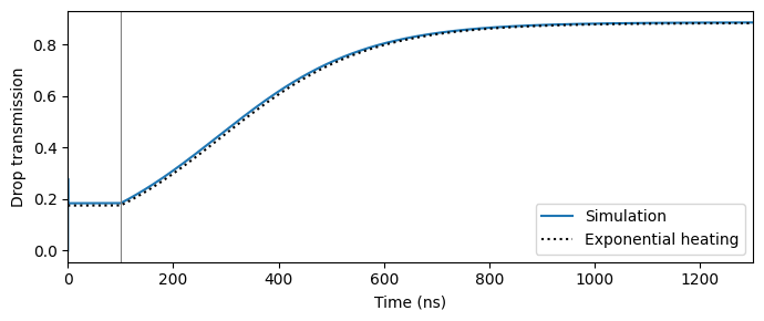
The 0.1 mW heater raises the ring temperature by 3.6 K and moves the resonance by about one linewidth. The drop transmission follows the temperature through the Lorentzian line shape, so it rises slowly at first, while the resonance is still far from the laser, and reaches the peak after about five thermal time constants. The ring itself responds within picoseconds, so the drop power follows the temperature without delay.

The tuning efficiency of 2.4 nm/mW corresponds to \(\eta = 1\), and it is high because the thermal impedance of this small ring is high. A heater that tunes the same ring by 0.3 nm/mW would have \(\eta \approx 0.13\), and would be modeled with heater_resistance=1e3 / 0.13.

The heater also shares the thermal time constant. A real heater responds more slowly than optical self-heating, since its heat has to diffuse to the waveguide, and a single thermal node cannot hold both time constants. When the heater dynamics matter, for example in a thermal locking loop, set thermal_time_constant and thermal_capacity to match the effect that dominates the experiment.

Free carriers and self-pulsing

Now we add the fast effects. The material constants of silicon at 1550 nm are:

• \(\beta_\mathrm{TPA} = 0.81\) cm/GW, with \(\Gamma = 0.99\). Borghi et al. [4] computed this TPA confinement factor for their waveguide with a mode solver. TPA grows with the square of the intensity, so \(\Gamma\) weights the mode by \(\lvert E \rvert^4\). That weight is concentrated in the silicon core, so \(\Gamma\) is close to 1 although a sizeable part of the power travels in the oxide.

• \(\sigma_\mathrm{FCA} = 1.5\times10^{-17}\) cm² and \(\sigma_\mathrm{FCD} = -9.5\times10^{-21}\) cm³, per electron-hole pair.

• \(n_2 = 4.5\times10^{-18}\) m²/W.

The effective area follows from the mode volume \(V = 4.87\) µm³ used by Borghi et al. [4] for the carriers, \(A_\mathrm{eff} = V/L\).

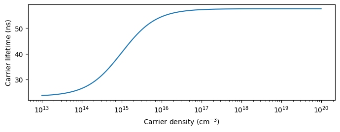
The carrier lifetime of a silicon waveguide is set by recombination at defects, the Shockley-Read-Hall (SRH) process, and it depends on the carrier density. srh_lifetime tabulates the SRH lifetime over a range of densities and returns an Interpolator that can be passed to carrier_lifetime directly. With its default trap parameters the lifetime rises from the electron lifetime \(\tau_n\) = 22.5 ns at low injection to \(\tau_n + \tau_p\) = 57.5 ns once the carrier density exceeds the background doping of 10¹⁵ cm⁻³.

# Tabulate the SRH carrier lifetime over the carrier density (1/m^3)
densities = np.geomspace(1e19, 1e26, 500)
lifetime = pf.srh_lifetime(densities)

# Plot the lifetime against the carrier density in 1/cm^3
fig, ax = plt.subplots(figsize=(7, 2.8), tight_layout=True)
ax.semilogx(densities * 1e-6, lifetime(densities) * 1e9)
ax.set(xlabel="Carrier density (cm$^{-3}$)", ylabel="Carrier lifetime (ns)")
plt.show()

# Set the nonlinear material constants of silicon
kerr_index = 4.5e-18  # Kerr coefficient (m^2/W)
tpa_coefficient = 8.1e-12  # Two-photon absorption coefficient (m/W)
fca_cross_section = 1.5e-21  # Free-carrier absorption cross-section (m^2)
fcd_coefficient = -9.5e-27  # Free-carrier index change per carrier density (m^3)
confinement = 0.992  # Fraction of the mode in the silicon core

# Compute the effective area from the mode volume (m^2)
mode_volume = 4.87e-18  # Mode volume (m^3)
effective_area = mode_volume / (length * 1e-6)
print(f"Effective area: {effective_area * 1e12:.3f} um^2")

# Create the ring with every nonlinear effect at the real thermal time constant
silicon_ring = pfa.nonlinear_ring(
    **ring_kwargs,
    dn_dT=dn_dt,
    effective_area=effective_area,
    kerr_index=kerr_index,
    tpa_coefficient=tpa_coefficient,
    fca_cross_section=fca_cross_section,
    fcd_coefficient=fcd_coefficient,
    confinement=confinement,
    carrier_lifetime=lifetime,
    thermal_time_constant=tau_th,
    thermal_capacity=c_th,
)

Effective area: 0.111 um^2

FCD and heating move the resonance in opposite directions and on very different time scales. For a laser on the red side of the resonance, this makes the stationary state unstable at high power [3]:

1. On the hot branch the resonance sits just above the laser. The ring keeps heating, and the heating pulls the resonance down towards the laser.

2. Once the resonance reaches the laser, any small loss of stored energy lowers the carrier density. This removes part of the FCD shift, so the resonance moves further down and the ring loses more energy. The runaway takes nanoseconds and leaves the resonance below the laser, with little light in the ring.

3. With little light in the ring, the carriers recombine and the ring cools with \(\tau_\mathrm{th}\), which moves the resonance back up. When it passes the laser, the stored energy builds up, the carriers generated by TPA push the resonance back above the laser, and the cycle repeats.

The period of the resulting oscillation is set mainly by the cooling, so it is of the order of \(\tau_\mathrm{th}\). The next cell drives the ring with 9 dBm at 25 GHz below the resonance for 5 µs. The run is about 15 million time steps, so it is stepped in chunks: the time stepper keeps its state between calls to step, so consecutive chunks form one continuous run. From each chunk we keep every 100th sample of the drop and through powers. This cell takes several minutes.

# Set the operating point
p_pump = 1e-3 * 10 ** (9 / 10)  # Input power: 9 dBm (W)
f_laser = f_res - 25e9  # Laser 25 GHz below the resonance

# Set the record length, the chunk size and the decimation of the stored output
duration = 5e-6  # Record length (s)
chunk = 500000  # Time steps per call to step
keep = 100  # Keep one of every 100 samples

# Set up the time stepper and the CW input for one chunk
time_stepper = silicon_ring.setup_time_stepper(
    time_step=time_step, carrier_frequency=f_laser, show_progress=False
)
a_in = pf.TimeSeries(
    {"P0@0": np.full(chunk, np.sqrt(p_pump), dtype=complex)}, time_step
)

# Step the ring chunk by chunk, keeping the decimated drop and through powers
drop_pulsing, through_pulsing = [], []
for _ in range(int(duration / time_step) // chunk):
    outputs = time_stepper.step(inputs=a_in, show_progress=False)
    drop_pulsing.append(np.abs(outputs["P2@0"][::keep]) ** 2)
    through_pulsing.append(np.abs(outputs["P1@0"][::keep]) ** 2)
drop_pulsing = np.concatenate(drop_pulsing)
through_pulsing = np.concatenate(through_pulsing)

# Build the time axis of the decimated record
t_keep = np.arange(drop_pulsing.size) * keep * time_step

# Find the period from the strongest line of the spectrum of the second half
tail = drop_pulsing[drop_pulsing.size // 2 :]
spectrum = np.abs(np.fft.rfft((tail - tail.mean()) * np.hanning(tail.size)))
freqs_pulse = np.fft.rfftfreq(tail.size, keep * time_step)
period = 1 / freqs_pulse[1 + np.argmax(spectrum[1:])]
print(f"Self-pulsing period: {period * 1e9:.0f} ns")
print(f"Drop power: {tail.min() * 1e3:.2f} mW to {tail.max() * 1e3:.2f} mW")

Self-pulsing period: 605 ns
Drop power: 0.09 mW to 6.20 mW

The first plot shows the whole record, and the second one period of the steady oscillation.

fig, (ax1, ax2) = plt.subplots(1, 2, figsize=(7, 3), tight_layout=True)

# Plot the drop power over the whole record
ax1.plot(t_keep * 1e6, drop_pulsing * 1e3)
ax1.set(xlabel="Time (µs)", ylabel="Drop power (mW)")

# Plot one period of the drop and through powers at the end of the record
last = t_keep > t_keep[-1] - 1.2 * period
ax2.plot(t_keep[last] * 1e6, drop_pulsing[last] * 1e3, label="Drop")
ax2.plot(t_keep[last] * 1e6, through_pulsing[last] * 1e3, label="Through")
ax2.set(xlabel="Time (µs)", ylabel="Power (mW)")
ax2.legend(fontsize=7)
plt.show()

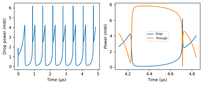
After a first transient of about a microsecond, the ring settles into a periodic oscillation with a period of about 600 ns. One period shows the phases described above:

• a low level of the drop power for most of the period, while the resonance sits below the laser and the ring cools,

• a short spike when the cooling brings the resonance up through the laser, followed by a fall to an intermediate level as the carriers generated by TPA push the resonance above the laser,

• a slow rise, over about 130 ns, while the heating pulls the resonance back towards the laser, and then the collapse when the resonance reaches it.

The through port shows the same dynamics inverted, since the light that is not dropped continues along the input bus.

Self-pulsing appears only within a window of input power and detuning: at lower power the stationary state is stable, and a laser on the blue side of the resonance does not produce it. Sweeping f_laser and p_pump in the cell above maps that window. The Kerr term makes little difference here, since the Kerr index change in silicon is small against FCD. In a silicon nitride ring, which has no TPA, the Kerr term and heating are the only nonlinearities; for such a ring set tpa_coefficient, fca_cross_section and fcd_coefficient to zero.

Summary

• pfa.nonlinear_ring is a single-bus or add-drop ring for time-domain simulations, built on pf.RingTimeStepper. The Kerr effect, TPA, free carriers, self-heating and a resistive heater are enabled by setting their arguments.

• At low power it matches the linear pf.RingModel, which is the quickest way to find the resonance and the linewidth. pf.RingModel.parameters_from_q converts quality factors into the ring’s loss and bus couplings.

• Self-heating makes the ring bistable for a laser on the red side of the resonance. The steady states depend only on the thermal impedance \(\tau_\mathrm{th}/C_\mathrm{th}\), so a quasi-static sweep can use a shorter time constant at the same impedance.

• heater_resistance adds an electrical port whose voltage heats the ring with power \(V^2/R\), acting through the same thermal impedance and time constant as the optical absorption. A heater that delivers only a fraction \(\eta\) of its power to the ring is modeled with the resistance \(R/\eta\).

• Free carriers from TPA push the resonance the other way on a nanosecond scale. Together with the slow heating this produces self-pulsing, with a period set mainly by the cooling of the ring. pf.srh_lifetime provides a density-dependent carrier lifetime for carrier_lifetime.