Optical Pulse

Not every optical source runs continuously. Pulsed lasers probe the impulse response of devices, carry return-to-zero data, and, as regular pulse trains, form the frequency combs behind optical clocks and parallel transmission. The OpticalPulseTimeStepper is the pulsed counterpart of the CWLaserTimeStepper: a source that emits Gaussian (or flat-topped super-Gaussian) optical pulses with a chosen energy, duration, and chirp, either as a single shot or as a periodic train, with the same intensity and phase noise mechanisms as the CW laser, covered in the CW Laser guide.

This guide characterizes single pulses, connects chirp to the pulse spectrum, builds pulse trains and their frequency combs, and generates pulsed on-off-keyed data.

Setup

import matplotlib.pyplot as plt
import numpy as np
import photonforge as pf
import photonforge.abstract as pfa

viewer = pf.live_viewer.LiveViewer()

LiveViewer started at http://localhost:61260

tech = pf.basic_technology()
pf.config.default_technology = tech

f0 = pf.C_0 / 1.55
time_step = 0.05e-12

Single Pulses

The abstract optical_pulse component is a source with a single optical port, so, like the lasers, it can be simulated on its own. The pulse is defined by its total energy and its duration width; note that width corresponds to the full width at half maximum of the field amplitude, so the intensity FWHM is shorter by \(\sqrt{2}\). If no offset is given, the pulse is automatically delayed so that it turns on smoothly from zero.

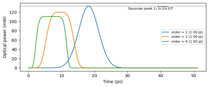
The order argument generalizes the shape to a super-Gaussian: higher orders flatten the top and steepen the edges at constant pulse energy. For the Gaussian pulse, the peak power follows from the energy and the intensity FWHM \(T\) as \(P_\mathrm{peak} = 2 \sqrt{\ln 2 / \pi} \, E / T\).

pulse = pfa.optical_pulse(energy=1e-12, width=10e-12)
viewer(pulse)

num_steps = 1024
t = np.arange(num_steps) * time_step

fig, ax = plt.subplots(figsize=(7, 3), tight_layout=True)
for order in [1, 2, 4]:
    source = pfa.optical_pulse(energy=1e-12, width=10e-12, order=order)
    time_stepper = source.setup_time_stepper(
        time_step=time_step, carrier_frequency=f0, show_progress=False
    )
    a = time_stepper.step(steps=num_steps, time_step=time_step, show_progress=False)["P0@0"]
    power = np.abs(a) ** 2
    energy = np.trapezoid(power, t)
    ax.plot(t * 1e12, power * 1e3, label=f"order = {order} ({energy * 1e12:.2f} pJ)")

# Peak power of the order-1 pulse from energy and intensity FWHM
fwhm_intensity = 10e-12 / np.sqrt(2)
peak = 2 * np.sqrt(np.log(2) / np.pi) * 1e-12 / fwhm_intensity
ax.axhline(peak * 1e3, color="k", linestyle=":", linewidth=1)
ax.text(30, peak * 1e3 - 8, "Gaussian peak $2 \\sqrt{\\ln 2 / \\pi} \\, E / T$", fontsize=8)
ax.set(xlabel="Time (ps)", ylabel="Optical power (mW)")
_ = ax.legend(fontsize=8)

Chirp and the Pulse Spectrum

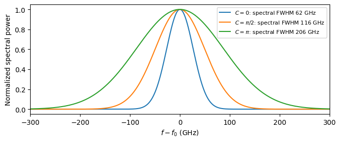
A transform-limited Gaussian pulse has the smallest spectrum its duration allows: the product of the intensity FWHM in time and frequency is \(2 \ln 2 / \pi \approx 0.441\). The chirp argument adds a quadratic phase \(C (t - t_0)^2 / (2 \sigma^2)\) across the pulse (like other phase-like arguments, \(C\) is specified in degrees, so \(C = \pi\) is passed as 180). An instantaneous frequency that slides across the pulse broadens the spectrum by \(\sqrt{1 + C^2}\) while leaving the power envelope untouched, exactly what dispersive propagation does to a short pulse.

chirps = {"$C = 0$": 0.0, "$C = \\pi/2$": 90.0, "$C = \\pi$": 180.0}

num_steps = 2**14
pad = 2**17
freq = np.fft.fftshift(np.fft.fftfreq(pad, time_step))

fig, ax = plt.subplots(figsize=(7, 3), tight_layout=True)
fwhm_spectral = []
for label, chirp in chirps.items():
    source = pfa.optical_pulse(energy=1e-12, width=10e-12, chirp=chirp)
    time_stepper = source.setup_time_stepper(
        time_step=time_step, carrier_frequency=f0, show_progress=False
    )
    a = time_stepper.step(steps=num_steps, time_step=time_step, show_progress=False)["P0@0"]
    # Zero-padded FFT of the envelope for a finely resolved spectrum
    spectrum = np.abs(np.fft.fftshift(np.fft.fft(a, pad))) ** 2
    spectrum /= spectrum.max()
    above = freq[spectrum > 0.5]
    fwhm_spectral.append(above.max() - above.min())
    ax.plot(freq / 1e9, spectrum, label=f"{label}: spectral FWHM {fwhm_spectral[-1] / 1e9:.0f} GHz")

ax.set(xlabel="$f - f_0$ (GHz)", ylabel="Normalized spectral power", xlim=(-300, 300))
_ = ax.legend(fontsize=8)

fwhm_intensity = 10e-12 / np.sqrt(2)
print(f"Time-bandwidth product at C = 0: {fwhm_spectral[0] * fwhm_intensity:.3f} "
      f"(transform limit: {2 * np.log(2) / np.pi:.3f})")
print(f"Spectral broadening at C = pi/2 and pi: "
      f"{fwhm_spectral[1] / fwhm_spectral[0]:.2f}, {fwhm_spectral[2] / fwhm_spectral[0]:.2f} "
      f"(analytic: {np.sqrt(1 + (np.pi / 2) ** 2):.2f}, {np.sqrt(1 + np.pi**2):.2f})")

Time-bandwidth product at C = 0: 0.440 (transform limit: 0.441)
Spectral broadening at C = pi/2 and pi: 1.86, 3.30 (analytic: 1.86, 3.30)

Pulse Trains and Frequency Combs

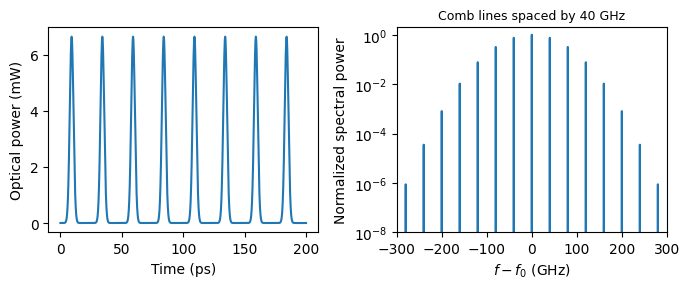
A positive repetition_rate turns the single shot into a periodic train, the time-domain picture of a mode-locked laser. In the spectrum, a periodic train of identical pulses is a frequency comb: discrete lines spaced by the repetition rate under the envelope of the single-pulse spectrum. The phase argument accepts a sequence applied pulse by pulse, and jitter adds RMS timing noise to the clock for realistic sources.

repetition_rate = 40e9
source = pfa.optical_pulse(energy=25e-15, width=5e-12, repetition_rate=repetition_rate)

# Record an integer number of pulse periods for a clean comb spectrum
periods = 64
num_steps = int(round(periods / repetition_rate / time_step))
t = np.arange(num_steps) * time_step

time_stepper = source.setup_time_stepper(
    time_step=time_step, carrier_frequency=f0, show_progress=False
)
a = time_stepper.step(steps=num_steps, time_step=time_step, show_progress=False)["P0@0"]

spectrum = np.abs(np.fft.fftshift(np.fft.fft(a))) ** 2
spectrum /= spectrum.max()
freq = np.fft.fftshift(np.fft.fftfreq(num_steps, time_step))

fig, (ax1, ax2) = plt.subplots(1, 2, figsize=(7, 3), tight_layout=True)
ax1.plot(t[: num_steps // 8] * 1e12, np.abs(a[: num_steps // 8]) ** 2 * 1e3)
ax1.set(xlabel="Time (ps)", ylabel="Optical power (mW)")
ax2.semilogy(freq / 1e9, spectrum)
ax2.set(
    xlabel="$f - f_0$ (GHz)",
    ylabel="Normalized spectral power",
    xlim=(-300, 300),
    ylim=(1e-8, 2),
)
_ = ax2.set_title(f"Comb lines spaced by {repetition_rate / 1e9:.0f} GHz", fontsize=9)

Pulsed Data

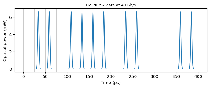
Setting prbs gates the train with a pseudorandom bit sequence, producing return-to-zero on-off-keyed data at the repetition rate: a pulse in the bit slot for a one, nothing for a zero. Together with jitter, rel_intensity_noise, and linewidth, this makes a realistic pulsed transmitter source without any modulator.

source = pfa.optical_pulse(
    energy=25e-15, width=5e-12, repetition_rate=repetition_rate, prbs=7, seed=0
)

num_bits = 16
num_steps = int(round(num_bits / repetition_rate / time_step))
t = np.arange(num_steps) * time_step

time_stepper = source.setup_time_stepper(
    time_step=time_step, carrier_frequency=f0, show_progress=False
)
a = time_stepper.step(steps=num_steps, time_step=time_step, show_progress=False)["P0@0"]

fig, ax = plt.subplots(figsize=(7, 3), tight_layout=True)
ax.plot(t * 1e12, np.abs(a) ** 2 * 1e3)
for k in range(num_bits + 1):
    ax.axvline(k / repetition_rate * 1e12, color="k", linewidth=0.5, alpha=0.3)
ax.set(xlabel="Time (ps)", ylabel="Optical power (mW)")
_ = ax.set_title(f"RZ PRBS7 data at {repetition_rate / 1e9:.0f} Gb/s", fontsize=9)

Summary

• pfa.optical_pulse emits Gaussian optical pulses defined by energy and width (the FWHM of the field amplitude; the intensity FWHM is width\(/\sqrt{2}\)), with order flattening the shape into a super-Gaussian and offset positioning the first pulse.

• A transform-limited pulse satisfies the time-bandwidth product \(2 \ln 2 / \pi\); chirp adds quadratic phase (specified in degrees) that broadens the spectrum by \(\sqrt{1 + C^2}\).

• repetition_rate produces periodic trains whose spectra are frequency combs spaced by the repetition rate; phase takes per-pulse values and jitter adds clock noise.

• prbs gates the train into return-to-zero on-off-keyed data, forming a complete pulsed transmitter source.

• frequency, rel_intensity_noise, and linewidth behave exactly as in the CW Laser guide, and a short pulse also serves as the optical impulse for response measurements, complementing the electrical impulse technique shown in the other guides of this section.